The New Physics
Closing in On the Answer
 Doug
Doug
 2 Comments
 Email
Email Print
PrintIn the previous entry, I explained how we use the 3D space/time oscillations of our theory, or the fundamental SUDRs and TUDRs, to form S|T units that are “preons,” triplets of which are used to build quarks and leptons and their anti-particles, as described in the LST standard model of particle physics.
Only the first family of the three families of the standard model have been modeled with the S|T preons, since it has seemed more important to concentrate on the periodic table of elements, and the atomic spectra, than to spend time considering the other two families of the standard model. However, this may have been a mistake.
In correspondence with Dave (see comments), who seems to have an uncanny ability to discover new relationships between known physical constants, I have learned that there is an important number that some researchers in the LST community refer to as “that damned number,” because, as unlikely as it might seem, it keeps popping up in the study of particle masses (see discussion here.)
Coincidentally, the same number, 2/9, plays an important part in Larson’s RSt, as he explains here. In the LST work that Dave has been contributing to, where he makes some amazing clarifications, the number 2/9 relates the charged lepton masses of the standard model with each other, as described by Carl Brannen in several papers, but probably most simply, starting with this one.
In the meantime, I’ve also discovered “that damned number” in the S|T preons. It turns out that, when we include the inner and outer balls defined by Larson’s Cube (LC), we are constrained to the inverse of the square root of 2/9 in the volume formula for the SUDR and TUDR.
I say constrained, because, regardless which measure we choose for the unit, or metric, of the LC, the geometry defines two, inverse, volumes, containing this number: The unit LC defines the volume of the outer ball, which always has a radius of the square root of 2, and the inverse of this ball, which has a radius of the inverse of the square root of 2.
Of course, this conforms to our new number system and bodes well, given the Le Cornec ionization energy (IE) analysis of the atomic spectra of the periodic table, which is based on the ratio of the square root of Hydrogen’s IE, to the square root of the IE’s of the other elements.
All this is very motivational, to say the least, and has lead me to suspect that the LC can be used to unravel these fundamental relationships, in our RST based theory.
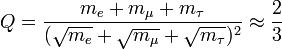
But now Dave has shown me that a conversion constant can be derived from Carl Brannen’s and/or Hans de Vries’ studies of the ratios of lepton masses, based on the Koide formula, which also incorporates squares and square roots. It’s a very simple formula that divides the sum of the masses of the charged leptons (electron, muon and tau), by the square of the sum of their square roots.
What Carl did was to use the curious fact that the formula can be related to spin matrices, and his equivalent density matrices, to find mass ratios that can then be algebraically “back calculated” from the known energy values of the leptons to find conversion constants. For instance, Dave showed me that the conversion constant calculated using the electron mass-energy goes like this:
(1 + sqrt2*cos(2*pi*1/3 + 2/9))^2 = 0.001628115,
where the 1/3 term is used for the electron, because it is the first generation charged lepton. For the muon, or the second generation charged lepton, we would use 2/3, and for the tau we would use 3/3, in the formula.
Now with these values, we can “back calculate” the conversion constant for the mass of a given charged lepton. For instance, for the electron:
0.001628115093 * X = .511 MeV
X = .511 MeV / 0.001628115093
X = 313.8598753 MeV
In fact, it turns out that this calculation from the formula yields the same 313.8 Mev conversion constant for all three masses. At this point, Dave decided to call this common constant the “unit lepton mass,” something that would probably not be appreciated as much by the LST community, as by the RST community, which recognizes the crucial importance of the unit value as lying between reciprocals.
Larson, for example, went to some length to point out to the LST community that E = mc2 does not mean that mass and energy should be regarded as the same, but it means that a quantity of mass is the equivalent of a quantity of energy: the one can be converted into the other by the conversion constant, c2, but they are two quantities of different physical dimensions and therefore two different entities altogether, which have something that is more fundamental in common - namely, motion.
In this case, the “back calculated” mass constant enables Dave to fit the results of the lepton mass formula into a reciprocal relation, via the squaring operation, which is the last step of the formula; that is, if the penultimate output of the formula happened to be 1, for some reason, squaring 1 and multiplying the result by the constant would not change the constant: clearly, the result would be the constant itself.
However, squaring the actual penultimate results of the formula yields values above and below the imaginary unit value of the formula, producing the reciprocal relation around the constant. Dave explained it to me this way:
0.0403499082^2 = 0.001628115 <— squaring result with the 1/3 term (electron) << 1
0.5802119201^2 = 0.336645872 <— squaring result with the 2/3 term (muon) < 1
1.000000000^2 = 1000000000 <— squaring result with unknown term (imaginary) = 1
.379438172^2 = 5.661726014 <— squaring result with the 3/3 term (tau) > 1
which is an amazing insight, I think. It tells us that the lepton mass formula, which requires “that damned number,” 2/9, no doubt incorporates a reciprocal relation of some kind. Not that the lepton masses themselves are somehow reciprocal, but that the reciprocity of factors determining them may play an unrecognized, but crucial role.
There’s more to explain here than I can include in one post entry, so, as a start, I will focus on the physical meaning of the mysterious number, 2/9, which, in the LST-based findings, has no physical meaning, but which appears in the volume formula of the oscillating S|T units of our RST-based physical theory here at the LRC.
The calculation of the two, reciprocal, unit displacement volumes, the SUDR and the TUDR, is straight forward enough. We begin with the LC, which is a 2x2x2 stack of 8 unit cubes. The outer ball that just contains the LC necessarily has a radius of 21/2. To find the inverse of this ball, which necessarily has a radius of 1/21/2, we only need to construct a second LC inside the inner ball, which is just contained inside the first LC. This second, smaller, LC is also a 2x2x2 stack of 8 cubes, but each cube necessarily has length, width and height of 1/21/2, instead of 1.
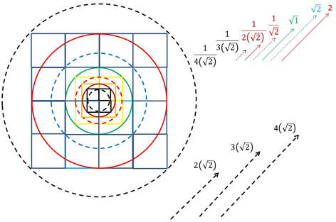
Figure 1. 2D View of Nested LCs and Associated Outer and Inner Balls. The radius of the outer ball (dashed blue circle) of the unit LC is 21/2, while its inverse (dashed red circle) is 1/21/2. The volume of the outer ball is eight times the volume of its inverse, which is π(2/9)1/2 . The ratio of the difference between the volume of the inner ball and the volume of the outer ball, and the difference between the volume of the inner ball and the volume of the inverse of the outer ball is 81/2.
The volume formula is 4/3 π * r3. Thus, the volume of the smaller, SUDR, ball, the inverse of the outer, TUDR, ball, is 4/3 * π * 1/21/2 = 1/4.51/2 * π. But the inverse of 4.5 is 2/9, so the volume of the SUDR turns out to be: π(2/9)1/2. The volume of the TUDR, based on its radius of 21/2, is 8 times this value, or 8π(2/9)1/2.
Hence, the number, 8, or 23, is the 3D number system’s equivalent of the 0D number system’s number 4, or 22; that is, whereas in the 0D scalar number system (what we could call the digital number system), the ratio of the two, inverse, unit displacements is
(2/1)/(1/2) = 4,
in the 3D pseudoscalar number system (what we could call the analog number system), the corresponding ratio of the two, inverse, unit displacements is
((21/2/1)3/(1/21/2)3 = 8.
However, whereas in the digital number system, the difference between the unit 1 and the unit 2 is 2-1 = 1 and the difference between the unit 1 and the inverse of the unit 2, 1/2, is
1-1/2 = .5,
and their ratio is
1/.5 = 2, or 21,
in the analog number system the corresponding ratio of differential volumes is
(8π(2/9)1/2)-(4/3 * pi)/(4/3 * pi)-(π(2/9)1/2) = 81/2, or (21/2)3.
Therefore, there is a symmetry in the pseudoscalar number system that is not found in the scalar number system.
In other words, in the operational interpretation of number, which allows us the quotient AND the difference interpretations of numbers, (giving us fractions of a unit as inverses on the one hand, and negative whole numbers as inverses on the other hand), the digital number system’s two fundamental ratios are 22 and 21, respectively, introducing a dimensional asymmetry between the two operational interpretations, but in the corresponding fundamental ratios of the analog number system, they turn out to be 23 and (21/2)3, wherein the dimensional symmetry is preserved between the two operational interpretations of the 3D numbers.
Right now, the significance of this is mostly academic, and probably should have been explained in the New Math blog of the LRC, but, given the teasing information that Dave keeps providing us and the beauty of the simplicity of these findings, one is reminded of the old saying: where there is smoke, there is fire.
More later.
Update: To clarify: The equation of the ratio of differential volumes should be written:
((8*pi*sqrt(2/9))-((4/3)*pi))/((pi*sqrt(2/9)-((4/3)*pi))) = sqrt(8),
where the unit volume is ((4/3)*pi*13) and the order of subtraction in the numerator is reversed from that in the original equation.
The Impact of Inverses
At the end of the previous entry, I promised to show how the neutron is the inverse of the proton. Actually, the LST community’s abstract concept of quantum “isospin” treats them as inverses, even though they differ by charge and by a very small difference in mass.
Also, the LST’s concept of quarks provides a sense of the inverse composition of proton and neutron, since the proton consists of two up quarks and a down quark, while the neutron consists of two down quarks and an up quark.
In our case, since the difference between the quarks consists of differences between their three sets of discrete, inverse, oscillations, the preons forming them, we can quantify this net inverse relation by employing a schematic diagram to represent the combinations.
The up quark has two sets of 3D oscillations with one more TUDR (2) than SUDR (1), together with one balanced set consisting of one SUDR and one TUDR. Hence, we can replace it with the number 2, because 1+1+0 = 2.
The down quark consists of two balanced sets and one unbalanced set with two SUDRs and one TUDR. We can therefore replace it with the number -1, because -1+0+0 = -1. Consequently, representing the proton with two 2s, for its two up quarks, and one -1, for its one down quark, placed at the three vertices of a triangle, we get 2, 2, -1, while doing the same thing for the three quarks of the neutron will give us a -1, -1, 2 pattern, which is the inverse pattern of the proton.
Using the same procedure with the electron, which has three unbalanced sets of 3D oscillations, all unbalanced to the SUDR (red) side, we get -1 + -1 + -1 = -3. Thus, the electron “neutralizes” the excess positive sum of the proton’s quark numbers ((2+2+(-1)) + ((-1)+(-1)+(-1)) = 0), while, of course, the sum of the neutron’s quark numbers is already 0.
Thus, it all comes together nicely in the schematic of triangles, which represents the net oscillations, after a fashion, as shown graphically here.
This development was so encouraging when it first emerged two and half years ago, that I was sure we would be able to continue it and reach our goal of tying our preon version of the standard model of particle physics, with our 4n2 version of the periodic table, the Wheel of Motion.
This would be an important achievement, since it would be the first time in history that an alternative to the LST community’s quantum mechanics and its wave equation, based on the concept of rotation, would have emerged.
Alas, however, crossing the bridge between the preon model and the Wheel of Motion has been more difficult than imagined. As described here, it appears that we have to follow Hamilton’s work with rotation and accept the fact that the number four plays an essential role in the combining of our preons to form the correct series of elements in the Wheel of Motion.
While it’s true that the inverse numbers in the schematics of the proton and neutron work nicely to combine them into combos that have interesting properties, including spin, the Pauli Exclusion principle and the concentration of numbers at the center of the combo, with numbers spread out at the periphery, the fact is, there is no mechanism for limiting the preon numbers, in the same way that the correspondence with vectorial motion in rotations limits the quantum numbers. It’s the limit that we are lacking. The question boils down to this: “What is the ‘n’ in the “4n2” relationship of the Wheel of Motion?
Schematically, we can build an atom by placing the proton and neutron together as shown for deuterium, helium and lithium in figure 1, below:
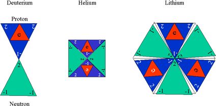
Figure 1. Building Atoms from Preons
As can be seen from figure 1, when represented with the three vertices of a triangle, schematically, the up and down quark and electron preons, form combinations that we can identify as hydrogen (the proton and electron combo without a neutron (not shown separately)), as deuterium (one hydrogen and one neutron), as helium (two hydrogen and two neutrons) and as lithium (three hydrogen and three neutrons). The electron is shown schematically in two states: The black letter “e” represents one state (on top of the proton triangle), while the white letter “e” represents the other state (on the bottom of the proton triangle).
While this enables us to find parallels with the four quantum numbers schematically, if not physically, the problem is there is no variable ‘n’ that can be identified that corresponds to the radius of an electron shell in the quantum mechanical model of the LST, the primary quantum number ‘n’ in the 2n2 relations of the periodic table.
This has driven me back to the beginning, to take another look at the fundamental 3D oscillations, the SUDRs and TUDRs. While we have only considered one family of the standard model’s quarks and leptons, it has always been evident that we could probably derive the second and third families by adding to the number of SUDRs and TUDRs in the preons, while maintaining their ratios. It was left at that, because it was assumed that connecting the Wheel to the preons was not related to the other families, and that part of the development could therefore be delayed, until later.
However, this appears to have been an error. I’ll explain why next time.
The Next Step
Ok, in the last entry, I explained how, like Hamilton’s quaternion solution, which enabled him to go from 2D geometric rotation to 3D geometric rotation, by exploiting four mathematical dimensions, rather than the three he thought it would take, our mathematical solution must be based on the number four, rather than the number 3, in order to go from the triplets of the preons to the quads of the periodic table of elements (4(12 )= 22= 4 is the initial magnitude of the Wheel of Motion version of the periodic table).
The reason this appears to be the case is that we must use the radius of the balls in Larson’s cube, rather than the cubes (i.e. the continuous numbers rather than the discontinuous). The preons use the cubes, since they are simply counting the relative number of inverse oscillations that are combined together in the preons.
However, just as our numbers on the new number line are not equal, given the quotient interpretation, even though they are equal, given the difference interpretation, so too our 3D oscillations (SUDRs & TUDRs) can represent equal, but opposite, space/time and time/space displacements from unity (i.e. equal up and down displacements from no displacements), even though they are not equal in magnitude (speed). The magnitude of the upper one (blue) is four times the magnitude of the lower one (red).
This means we must count the total number of oscillations, red and blue, in a given preon, and then apply the quotient interpretation of the numbers to get the relative magnitudes, For instance, the up quark has two blue and a green in the midpoint of its three S|T units. Since the color green of the midpoint indicates a balance of red and blue, and the color blue of the midpoint indicates an imbalance of one more blue than red, we have a total five blues and three reds in the up quark (we have to count the two, opposing, units that balance the initial S|T unit before it is unbalanced in one or the other “direction.”)
On the other hand, the down quark has three green and one red, so it has a total of three blues and four reds. Now the proton consists of two up quarks and one down quark, while the neutron consists of one up quark and two down quarks. Hence, the red:blue ratio for the proton is 10:13, while for the neutron it’s 11:11. But when we add the 6 red and 3 blue of the electron to the total of the proton, its ratio is changed to 16/16.
Adding up the total blue:red magnitudes for the proton, we get (32/1):(16/2) = 64/16 = 4, while for the neutron we get (22/1):(11/2) = 44/11 = 4. This is a surprising, but welcome result, since it again conforms with the LST’s standard model of particle physics: The proton and neutron only differ by the positive charge of the proton and a slight difference in mass. The trouble is, the difference in mass is not in accord with the standard model. Whatever mass might turn out to be in our RST theory, it seems unlikely that the higher numbers of the proton would make it slightly lighter than the neutron, rather than the other way around.
Nevertheless, the good news is that, when we get to the atomic level, our triplets of S|T preon units turn out to be quads of S|T atomic units, which are ready to be compounded into the periods of the Wheel of Motion.
Now, the next step is to treat the 4 of the proton and the 4 of the neutron as inverse numbers, in the sense that the patterns of their constituent preons are inverses. I’ll explain how that works in the next post.
Another Brougham Bridge Moment?
There is an obscure plaque on the Brougham Bridge in Dublin, which reads:
According to Wikipedia, “mathematicians from all over the world have been known to take part in the annual commemorative walk from Dunsink Observatory to the site [of the plaque]. Attendees have included Nobel Prize winners Murray Gell-Mann, Steven Weinberg and Frank Wilczek, and mathematicians Sir Andrew Wiles and Ingrid Daubechies.”
I’ve referred to the story of Hamilton’s discovery of quaternions many times over the years, because Hestenes makes it so interesting. At the point in time that I discovered Hestenes and his GA, I had no idea what quaternions even were. One evening at an ISUS conference in SLC, John Pratt tried to explain them to a group of us that stayed up until midnight to learn about them.
The crux of Hamilton’s “flash of genius” was the realization that, to move from 2D algebra (what has become known as the algebra of complex numbers) to 3D algebra (now known as quaternions, meaning four), requires four dimensions (here the word “dimensions” is to be taken in the sense of the mathematician, not in the normal geometric sense).
Hamilton had been trying to find a 3D algebra based on 3 mathematical dimensions, which he thought should require three independent numbers to define it (see Larson’s discussion of mathematical dimemsions here). It was at the bridge, walking with his wife, that he suddenly realized that a 3D algebra requires 4 dimensions, or 4 independent numbers to define it, not 3, as one would think.
Hamilton’s fascination with his quaternions from that point on kept him from doing anything else. He was obsessed with them until the day he died, but they eventually fell into obscurity and his complete devotion to them was generally regarded as a tragic waste of the genius’ career.
That’s because everything that needed to be done in electrical engineering and theoretical physics could be done with the 2D algebra of complex numbers. It wasn’t until the last half of the 20th Century, that engineers began to see an advantage to the 3D algebra, mainly in robotics.
Some few theoretical physicists have sought to employ quaternions and even the eight dimensional algebra of octonions in their theoretical work, but these efforts have not enjoyed a lot of success. So, why are Nobel Prize winning physicists and mathematicians so interested in this commemoration of Hamilton’s insight?
It’s because of Clifford algebras and the binomial expansion, which captures the reality of three (geometrical) dimensions and the two “directions” inherent in each of those dimensions: Counting the “directions” of nature we get 20 = 1, 21 = 2, 22 = 4 and 23 = 8, the four numbers of the tetraktys, which constrains Euclidean geometry and should constrain theoretical physics, but doesn’t, because mankind can’t explain the so-called elementary particles of nature and all their interactions, within its three dimensions. They need extra dimensions, because the “point,” and the three dimensions of physical reality, are not compatible in their theories.
Well, we have struggled within the tetraktys as well, but have embraced its constraints due to the second fundamental postulate of the RST. But just as the LST community is stuck, in their theoretical development, so are we. And it turns out that we are stuck, not at the 0D point, but where Hamilton was stuck: We have been trying to use three independent mathematical dimensions to understand motion in three geometric dimensions, but it takes four to do it!
Recall that in our preon model of the standard model of particle physics, formed from S|T units, which are formed in turn from the SUDRs and TUDRs, or the initial 3D space oscillations and 3D time oscillations, deduced from the fundamental postulates of the RST, we describe bosons (S|T doublets) and fermions (S|T triplets). The triplets form the quarks and the leptons, which, of course, we use to form the atomic elements of the periodic table (see Wheel of Motion), but based on their RST scalar motion values, not the vectorial motion values of the LST.
In each of these preons, we use three colors to represent the space/time and time/space displacements of the S|T and T|S units. For instance, the up quark triplets contains one green and two blue S|Ts, while the down quark triplet contains two green S|Ts and one red S|T, as shown below in figure 1.


Figure 1. The Three S|T Units of the Up and Down Quark Triplets
The red and blue endpoints indicate that the S|T (red) and T|S (blue) units are inverses (red is a “lower” displacement, a value below 0 displacement, while blue is a “higher” displacement, a value above 0 displacement). The colors of the midpoints indicate the ratio of S|T to T|S units. A green midpoint color denotes a 1:1 ratio, while blue denotes a 1:2 ratio and red denotes a 2:1 ratio.
It’s important to understand that these diagrams of the relative displacements do not contain all the information we would like to convey. For instance, since the actual physical oscillations are 3D, they would have to combine as balls, not lines (see here).
But two partially merged balls necessarily combine as a 1D entity (the line between their origins at their centers), while three partially merged balls necessarily combine as a 2D entity (the area defined by the plane formed from the three conected points of their origins). Moreover, there is no way to partially merge a fourth ball to change this geometry from the 2D area to a 3D volume, except by placing it on one side, or the other, of the three-ball plane.
This works out nicely in some ways, but when we completely merge the balls, this Euclidean geometry disappears. The question we’ve pondered has always been how far are the balls separated and how do we determine that distance? But with the new view of the 3D oscillation explained in the FQXI essay, the doubt arises as to why they even need to be partially merged. Maybe the S|T units are completely merged with the T|S units and, if this is true, how do we interpret the binding together of the red and blue entities?
It’s still true that the relative displacement from the perspective of each of the two displacements is akin to the balance scale: if the left is lower than the right from one perspective, then the opposite is true from the inverse perspective (if the left end of a teeter-totter is observed from the side view to be lower than the right end, then if the observer crosses over to the other side of the teeter-totter, turning around to view it from the opposite “direction,” the right end will be lower than the left end, even though it’s the observer’s right and left that have been swapped, not the teeter-totter’s).
However, in comparing two relative displacements (i.e. two teeter-totters), one displaced in the opposite direction of the other, i.e. 2:1 and 1:2, there are four points of comparison, which are the four endpoints of the two teeter-totters.
We can illustrate this with the teeter-totter, or lever analogy. If two levers are on the same pivot point mid-way along their length, with equal weights on each of their respective endpoints, they will be balanced in the horizontal, but if there are two of the equal weights on one end, and one on the other, the lever will not lie horizontally, but diagonally, and if the relative imbalance of the two levers is opposed, then they will lie in inverse diagonals, forming an X pattern, when viewed from the side.
Now, the question is, if the X pattern represents the relation (s:t):(t:s) and (s:t):(t:s), or two red-blue sets of the three in a triplet, then how do we include the third set in this same ratio? The answer is, I believe, we don’t. Just as Hamilton could not multiply triplets, but had to add a fourth mathematical dimension, we can’t compare three S|T units. In order to compare four S|T units, they must be combined as two sets of orthogonal Xs.
Fortunately, the two sets of Xs correspond to the eight corners of Larson’s cube, our 3D geometry generated by scalar motion, which just happens to perfectly integrate Euclidean geometry and our new algebra through the tetraktys. But now we need to ask, “Won’t this change in the fundamental combinations of S|T units ruin the three-fold symmetry of the preon model?”
Happily, it won’t. Not if its mathematical symmetry is interpreted geometrically, it won’t; That is, Larson’s cube can be extended (or unbalanced if you will) in each of its three dimensions, depending upon the relative number of its constituent S|T units in the three dimensions, which should, hopefully, enable us to preserve the existing preon model, while now building it by proceeding from 0D, to 1D, to 2D, to 3D, in the three iconic steps of the tetraktys.
This is an exciting advance in our development, if I’m not mistaken. Now, if I could only find a stone bridge to carve!
3D Oscillations
In writing the essay for the latest FQXi Contest, “Is Reality Digital or Analog?” I argued for the necessity of 3D time on the basis of space/time conservation; that is, space can’t increase, in the observed 3D spatial expansion, outside gravitational limits, without violating the law of conservation.
In the case of the postulated 3D space/time oscillation, we face double jeopardy from this law, as the volume of space, created during the expansion, disappears upon contraction to zero. “Where did it come from? Where did it go?”
Of course, the immediate conclusion is that it is transformed into its inverse, 3D time. This would not be surprising to students of the RST, but it must be startling to the LST community, who never seem to contemplate the possibility, even though it is a perfectly reasonable extrapolation from what we know about space and the laws of symmetry, which, after all, are laws of conservation, as Noether’s theorem proves.
However, what is surprising to me is that I realized that even I hadn’t thought about it before. The realization of its necessity didn’t strike me until I wrote the FQXI essay. I remember Larson saying something similar in the Preliminary version of The Physical Structure, but I have never spent the time to look for it.
Regardless, it appears to me that it is a significant insight that ought to play a central role in getting the RST comimunity more up to speed with the LST community, who, while theoretically challenged, is way ahead of us analytically.
The advantage they possess comes, in large part, from the physics of vector motion. When they faced the quantum mechanics challenge in the 20th century, they met it by finding ways to adapt the principles of vector motion to solve problems of scalar motion, something that they don’t recognize even to this day.
They are not happy with the QM situation, and they have tried many ways to correct the confusion that has resulted from it, but in the meantime we haven’t been of much help, unfortunately. Now, though, I think I see the way we can lead them to consider the physics of scalar motion, because the parallel between the two systems can be exploited in a way that was not possible before the change to Larson’s development of his RSt, which we introduced by taking exception to his concept of 1D “directiion” reversals, insisting that they had to be 3D.
This change, though so disruptive to ISUS, has lead to the conclusion that “scalar rotation” is an oxymoron. Physical entities rotate, translate and vibrate, but scalar ratios of space and time, which form physical entities, in the universe of motion, do not. They expand and they contract, or oscillate, like the zooming in and out in one, two or three dimensions, but that’s it. The elementary space/time entity, in the LRC’s development of RST theory, is a 3D oscillation that is a composite of 1D, 2D and 3D scalar motion.
Since unit speed is the datum of the universe of motion, the 3D oscillations are on either side of this speed, like the two sidebands of RF modulation. Taking the unit speed as s/t = 2/2, then the slower side is s/t = 1/2, while the faster side is s/t = 2/1. We have dubbed the slower one, the Space Unit Displacement Ratio, or SUDR, and the faster one the Time Unit Displacement Ratio, or TUDR.
By displacement, we mean that the oscillation of one aspect of the unit motion confines its magnitude to one unit of space or time, causing its reciprocal aspect to move forward two units for every cycle, thus displacing the unit ratio by one unit, in the appropriate “direction” (the same thing happens in rotation - it takes two units of time for every 360 degrees of rotation, a 1/2 ratio, even though we double the unit so we can speak in terms of cycles per unit of time).
However, until the composing of the essay, the oscillation of the SUDR (TUDR) was confined to space (time), with no consideration given to a law of space (time) conservation. It was in composing the essay, and thinking about the definition of a point of no extent, and an instant of no duration, a concept used in the LST community, but inconsistently, that the concept became clear: The 3D oscillation must transform into its inverse, just as the 2D vectorial oscillation does (see the FQXI paper here.)
What is clear now is that the 3D oscillation, when the inverse volume is included, can be described in the same way traditional oscillation is described, with something similar to the sine and cosine, or the ratio of orthogonal dimensions with the radius. The difference is that the magnitudes that constitute the sine and cosine, which are projections of the moving radius upon the two, inverse, dimensions, in the vectorial rotation, as the radius moves along the circumference, are changed to two actual magnitudes: The ratio of the these two, inverse, radii, the spatial and the temporal radii, the sum of which always equals 1, just as the familiar,
sin2Θ + cos2Θ = 1,
have the same relation, but just as they are, without the need to employ the Pythagorean theorem.
Indeed, we can say that, while the radius of rotation oscillation is fixed, but its angle changes, the radii of the expansion/contraction oscillation change, but their angle is fixed. As the angle of rotation increases from 0 to 360, the sine and cosine vary inversely:
Sine: 0 <—> 1 <—> 0
Cosine: 1 <—> 0 <—> 1
and as the progression of the 3D oscillation increases from 0 to 2, the temporal and spatial radii vary inversely, in exactly the same way:
Temporal radius: 0 <—> 1 <—> 0
Spatial radius: 1 <—> 0 <—> 1
The great thing about this is that there is no need to square anything to get the result, but that is not all. With this in hand, we can describe the 1D, 2D and 3D oscillations mathematically, together, or separately, and the 4π change (called “quantum spin”) per cycle falls out naturally (see table 1 in FQXI paper for details.) In addition, the 1D time/space oscillation, t/s, corresponds to the dimensions of electrical charge, the 2D oscillation, t2/s2, to the dimensions of magnetic flux, and the 3D oscillation, t3/s3 to the dimensions of mass.
Certainly, there is a mighty long way to go, but what a wonderfully simple, if prospective, solution it is.