The New Mathematics
Eleventh Post in the BAUT RST Forum
 Doug
Doug
 Post a Comment
We can gain a useful understanding of the conflict in the view of the dimensions of scalars, discussed above in terms of the definitions of mass and energy, and see how the existence of non-zero scalar dimensions actually clarifies how a physical scalar value such as energy can have non-zero mathematical dimensions, by studying the dimensional properties of the Greek tetraktys and comparing/contrasting the meaning of these dimensions in terms of vectors, Clifford algebas, and proportions, using the operational interpretation of number.
In the vector view of the tetraktys, the 20 points are scalar multipliers of 21 vectors, and a vector times a vector is another vector. So we have a resultant vector as the diagonal between two orthogonal vectors, or two non-parallel vectors, times the magnitude of a scalar, or this product times another vector times a scalar, etc. All the possible combinations and the mathematics for these vectors, in the tetraktys, are described by the vector algebra, using the numbers in its hypercomplex number system, the set of reals, complexes, quaternions and octonions.
In the Clifford algebra view of the tetraktys, used to formulate Geometric Algebra, the 20 points are again scalars, but vectors are directed, one-dimensional, lines, multiplied by the scalars, while the product of vectors is not another 1D vector, but a directed 2D bivector, or 3D trivector, again, multiplied by the scalars. All the possible combinations and the mathematics for these multivectors in the tetraktys are described in the Geometric Algebra, using the multi-dimensional number system, the set of zero, one, two, and three-grade blades.
By contrast, in the proportional view of the tetraktys, the “points” are also scalars, but, unlike in the previous views of 1D vectors and nD multivectors, the scalar in the proportional view is the source of the higher dimensional numbers, in the sense that all the higher-dimensional numbers in the tetraktys are expanded scalars, rather than rotated vectors, or multivectors. There are no vectors in this view, no vectors, no bivectors, and no trivectors, only “n-dimensional” scalars.
To illustrate how this works, we can use scalar values such as colors and walk them through the tetraktys. Each scalar value represents a relative proportion, which is either equal to, greater than, or less than, the reference proportion. We begin with the first element, at the top of the tetraktys (1), the 20 = 1 scalar, or the void. We assign the color black to it, a scalar value corresponding to a black “point,” if you will.
At the next higher dimension (11), 21 = 2 scalar, we can expand the “point” scalar value in two “directions” to form a 1D value corresponding to a geometric “line,” with three scalar values, representing the expansion of the black scalar, expanded to a scalar value, or “point,” on either side of black, to a red value, or “point,” on the left, and to a blue value, or “point,” on the right. The blue “point” is a scalar value of greater proportion than the black “point,” while the red “point” is a scalar value of less proportion than the black “point.” We will give the set of these three values, corresponding to a 1D geometric “line,” defined between the three scalar values, or “points,” the color green, representing the one-dimensional equilibrium established by its three scalar numbers.
At the next higher dimension, 22 = 4 scalar (121), again we have the zero-dimensional, black, “point,” but now we can expand it into two 1D scalar values, or “lines,” the new one of which we will color red. However, the difference in the color of the 1D values, represents a scalar difference in the symmetry of the two lines; one is symmetrical and one is not, the difference in symmetry defining two scalar “dimensions.”
There is a scalar difference of dimension between the red value and the green value, and this difference is manifest as the difference in the symmetry of the two 1D values; that is, the green 1D value is symmetrical, or balanced, but the red 1D value is unbalanced. Its symmetry is broken, we might say, in the red “direction,” representing the new, or second, dimension at this level. The product of these two 1D values, the green 1D “line” ^ red 1D “line”, is a yellow, “two-dimensional,” scalar value, corresponding to a geometrical “area.”
At the next higher dimension of the tetraktys, the 23 scalar on the fourth line (1331), we again have the 0D, black, “point,” but now we can expand it three ways, corresponding to the three vectors of the Clifford algebra tetraktys. One of these is the balanced scalar value, or the symmetrical 1D expansion, and the other two are the unbalanced scalar values, or two, 1D, non-symmetrical, expansions of the 0D black “point.”
The first, balanced, 1D value is again colored green, while the second 1D value, unbalanced in the red “direction,” is again colored red. The third 1D value, unbalanced in the blue “direction,” is colored “blue.” Now, we can combine each of the three, 1D, scalar values, with each of the others, so we have three combinations of two, 1D, scalar values, forming a 2D scalar value, and these three combinations correspond to the three, 2D, bivectors of the Clifford algebra tetraktys:
- green 1D “line” ^ red 1D “line” = yellow 2D “area”
- green 1D “line” ^ blue 1D “line” = cyan 2D “area”
- red 1D “line” ^ blue 1D “line” = magenta 2D “area”
Notice that, because these are scalar values, they are commutative; that is, the order of combining them makes no difference in the result. Now, at this, the bottom level of the tetraktys, there are also three more combinations, where we combine one of the three 1D values, with one of the three 2D values. However, there is only one result, regardless of the combinations, and it corresponds to the Clifford algebra, 3D, trivector, a “volume:”
- blue 1D “line” ^ yellow 2D “area” = white 3D “volume”
- red 1D “line” ^ cyan 2D “area” = white 3D “volume”
- green 1D “line” ^ magenta 2D “area” = white 3D “volume”
Figure 1 below illustrates the scalar tetraktys.
Figure 1. Scalar Tetraktys
Again, since these values are scalar values, their algebra is associative; that is, it doesn’t matter how the three, 1D, scalar values and the three, 2D, scalar values are grouped to form the one, 3D, scalar value, the result is always a white, 3D, volume.
Of course, the point is that the scalar combinations of the scalar tetraktys correspond to the combinations of the scalar values of the red SUDR, and the blue TUDR in the development of the physical theory that we are working on. The SUDR and TUDR, are initially joined together to form the green SUDR|TUDR combo. This combo (green 1D value) represents the one-dimensional, balanced, RN, the symmetry of which can be “broken” in two “directions,” by the addition of red SUDRs, and/or blue TUDRS, to the green symmetrical combo. Thus, we see that the units of scalar motion have three “dimensions,” and though these scalar “dimensions” are not the vectorial dimensions of Euclidean geometry, they are nevertheless consistent with three-dimensional mathematics. Not an insignificant result.
Once we understand this, we can see that the 1s running down the right side of the tetraktys in figure 1, have n “dimensions” (multicolors), while the 1s running down the left side of the tetraktys have 0 “dimensions” (black color), but they are all scalar values nonetheless.
Therefore, we see that the zero-dimensional units of mass, which we measure in kilograms, can also consistently be expressed as the three-dimensional units of scalar motion. Hence, all the physical dimensions reduce to consistent multi-dimensional units of space/time in two, reciprocal, scalar groups, when we provide the correct dimensions of the scalar values involved:
The energy group:
- mass = t3/s3
- momentum = t2/s2
- energy = t1/s1
The velocity group:
- inverse mass = s3/t3
- inverse momentum = s2/t2
- velocity = s1/t1,
where I’m explicitly indicating the one-dimensional values in the superscripts, for greater clarity. If 3D inverse mass is the mass of antimatter, then 2D inverse momentum is the momentum of antimatter, but it is also 1D velocity squared. So, multiplying 2D inverse momentum by 3D mass, yields 1D energy, as shown above, but, by the same token, multiplying 2D inverse mass (antimatter) by 2D momentum, yields 1D velocity,
v = s3/t3 * t2/s2 = s1/t1
So, then, what is 2D momentum and 2D inverse momentum? We know 2D momentum is a product of 3D mass and 1D velocity, so 2D inverse momentum must be the product of 3D inverse mass and 1D inverse velocity, but 1D inverse velocity is energy, therefore, 2D inverse momentum is the product of 3D inverse mass and energy, or
(p) = (m)*E = s3/t3 * t/s = s2/t2,
where the parentheses indicate inverse. So, though we don’t know what it means at this point, at least we have a consistent and fundamental definition of velocity times velocity, or velocity squared.
More to come on that later, but in the meantime, since force (a quantity of acceleration) is required to produce a 1D velocity of mass (2D momentum), an inverse force (a quantity of inverse acceleration) should be required to produce a 1D inverse velocity of 3D inverse mass (2D inverse momentum).
So, the next question is, then, what are force and acceleration? In the LST vectorial system, force and acceleration must be defined apart from mass and momentum, but in the RST this is not necessary.
In the new scalar system, force, is energy per unit space:
f = t/s * 1/s = t/s2,
while acceleration is velocity per unit time:
a = s/t * 1/t = s/t2.
So, force extended over space is energy,
E = t/s2 * s/1 = t1/s1,
while acceleration extended over time is velocity,
v = s/t2 * t/1 = s1/t1.
Further, force extended over time is momentum.
p = t/s2 * t/1 = t2/s2,
while acceleration extended over space is inverse momentum,
(p) = s/t2 * s/1 = s2/t2.
The only thing I want to emphasize at this point, is that these space/time dimensions are entirely consistent. Larson used this fact to great advantage, as you can see in Chapter 12 of “Nothing But Motion,” but he did so without knowledge of the scalar tetraktys. Now that we understand it better, we expect to be able to exploit these scalar equations of motion, both on the velocity side and on the inverse (energy side) of unity, to great advantage.
Stay tuned.
Excal

Toward a New Multi-Dimensional Scalar Number System
I’ve played around with number systems in the LRC’s New Math blog for years, but until a recent email exchange with my daughter Michele, I had not given it much thought for some time.
To my dismay, however, I started thinking about it again and, now, I cannot get it out of my mind. Readers of the blog might recall how one of my favorite topics in mathematics is how math, employed in theoretical physics, has developed historically.
I like to start with Sir William Hamilton and his discovery and fascination with quaternions (see here.) I first learned about it from David Hestenes, who more or less resurrected the idea of quaternions, in connection with his work on his Geometric Algebra.
Not being a mathematician, or even one inclined to the subject, my interest was driven by the implications of scalar motion, which seemed to me to be almost, if not entirely neglected by everyone except Dewey Larson and his followers.
Just before the disagreement within ISUS drove me to organize the LRC, I had given some thought to expressing the fundamental ideas of Larson numerically. I had this idea that the numbers 1/2, 1/1, 2/1 could be used to quantify the RST concepts of material and cosmic sector space and time displacements, as defined by Larson.
But soon, I realized that these one-dimensional numbers, if they were to be useful to express scalar motion entities, would have to be extended to multi-dimensional numbers, and this eventually led me to understand the great disconnect in modern number systems, as mathematicians tried to understand how to extend non-scalar motion, or vector motion, to multi-dimensions.
Ironically enough, it was Hamilton’s discovery of quaternions that led the way to the derailment, even though it was he who complained most eloquently about the use of so-called imaginary numbers, which eventually were to enable him to form quaternions, ironically enough. However, this use of imaginary numbers to increase the dimensions of ordinary, or scalar numbers, has led to pathological algebras, which I’ve talked about many times (e.g. see here.)
The fact is, only the algebra of one-dimensional numbers is non-pathological. The two-dimensional complex numbers lose the order property of scalar algebra, while the three-dimensional quaternions lose both the order property and the commutative property, and the octonians, which would be four-dimensional numbers, add associativity to the lost properties of multi-dimensional numbers.
Of course, if we consider scalars as zero-dimensional numbers, then complex numbers would be one-dimensional, quaternions would be two-dimensional and octonions would be three-dimensional, which would help clear up the understanding of non-mathematicians, with a geometric perspective, letting them relate the number systems to the corresponding geometrical concepts of point, line, area and volume.
However, the mathematicians look at numbers as algebraic operators, and they like to designate their dimensions in those terms, so an algebraic expression of complex numbers, with two terms, z = (a + bi), for example, is considered two-dimensional, and an expression of quaternions, with four terms, H = (a+bi+cj+dk), is considered four-dimensional, and one of octonions, with eight terms, a scalar number and seven imaginary numbers, is considered eight-dimensional.
Thus, unfortunately, the dimensions of algebra, lose their direct correlation with the dimensions of geometry, among the mathematicians. Nevertheless, we were able to show how the dimensions of numbers are indeed correlated with the dimensions of geometry, when viewed through the tetraktys and Larson’s Cube (e.g. see here.)
With all this as prelude, we come to the core of this blog entry: What can replace the multi-dimensional vector aglebra of today’s number systems, based on imaginary numbers? The answer is a multi-dimensional scalar algebra, based on ratio, which is the mathematical corollary to motion. In the set of zero-dimensional numbers, correlated with geometric points, the members of the set are the familiar rationals called integers and their inverses:
1/n, …1/3, 1/2, 1/1, 2/1, 3/1…, n/1
We can say that this set is based on multiples of the scalar unit 10 = 1, but what about a higher dimensional set based on multiples of the linear unit 11? What would its members look like? Or a set based on multiples of the square unit 12? What would its members look like? Or a set based on multiples of the cube unit 13?
The problem is that, in algebra, 10 = 11 = 12 = 13= 1 = (1x1) = (1x1x1), while in geometry, a unit point is a zero dimensional magnitude (10), differentiated from a unit line, which is a one-dimensional magnitude (11), differentiated from a unit area, which is a two-dimensional magnitude (12), and differentiated from a unit volume, which is a three-dimensional magnitude (13).
These multi-dimensional, geometric entities are not algebraically inter-operable. How do you multiply or divide a line times an area, or a point times a volume, or how do you add and subtract them from one another? You can’t, because the geometric dimensions of these units differ, while the dimensions, represented by the exponents in the corresponding algebra are not even dimensions in the same sense.
Unlike geometric dimensions, where each dimension is an orthogonal magnitude, the algebraic dimensions are not orthogonal magnitudes, but simply denote a number of factors in the expression of a mathematical operation.
However, if we recognize this difference, we can change the meaning of the exponents, so that:
0D = 10 = unit point
1D = 11/2= unit line
2D = 21/2 = unit area
3D = 31/2 = unit volume
This may appear to be a strange suggestion, but there is a way to employ these multi-dimensional numerical units, as geometric units, by utilizing a geometric theorem: the theorem of Pathagoras. Thus, given
n = 1, 2, 3, …, ∞,
Unit point = (12)1/2;
Unit line = (n2)1/2;
Unit area = (n2 + n2)1/2;
Unit volume = (n2 + n2 + n2)1/2.
On this basis, the members of the 0D scalar set, based on unit point numbers, are noted as before:
1) 1/n, …1/3, 1/2, 1/1, 2/1, 3/1…, n/1,
But the members of the 1D linear set, based on unit line numbers, are:
2) 1/n(12)1/2, …1/3(12)1/2, 1/2(12)1/2, (12)1/2/(12)1/2, 2(12)1/2/1, 3(12)1/2/1…, n(12)1/2/1.
The members of the 2D square set, based on unit area numbers, are:
1) 1/(n2+n2)1/2, …1/(32+32)1/2, 1/(22+22)1/2, (12+12)1/2/(12+12)1/2, (22+22)1/2/1, (32+32)1/2/1…, (n2+n2)1/2/1.
The members of the 3D cube set, based on unit cube numbers, are:
1) 1/(n2+n2+n2)1/2, …1/(32+32+32)1/2, 1/(22+22+22)1/2, (12+12+12)1/2/(12+12+12)1/2,(22+22+22)1/2/1, (32+32+32)1/2/1…, (n2+n2+n2)1/2/1.
If these multi-dimensional number sets turn out to have the properties required for mathematical groups, then their members should be able to be algebraically manipulated, with no pathology in the higher dimensions, as is now found in the higher dimensions of the legacy number system, based on imaginary numbers.
Some of the group properties are easily seen in the new sets. For instance, the identity element of all of them is equal to 1, which implies that multiplication by it will not change a member of the set. Also, a member of the set, when multiplied by its inverse is equal to 1. I think all the other group properties should hold as well, but I haven’t tested them to see.
For example, in the 2D case, the second element multiplied by its inverse element is:
Given x = sqrt(n), written in the form of the Pathagorean theorem, then:
(x)*(1/(x)) =
sqrt(2)*(1/(sqrt(2))) =
(12+12)1/2 * (1/(12+12)1/2 = ((12+12)1/2)/((12+12)1/2) = 1
Now, when each element is divided by its inverse, the 1D elements are squared, giving us the progression series,
1) e/(1/e) = e2 = 1, 2, 3, …n2,
while the 2D elements divided by their inverses produce the progression series:
2) e/(1/e) = e2 = 2, 8, 18, …2(n2),
and then the 3D elements divided by their inverses, produce the progression series
3) e/(1/e) = e2 = 3, 12, 27, …3(n2)
We can visualize these multi-dimensional, geometric numbers graphically, by drawing the unit ball inside the Larson cube, which just contains it, and drawing a second ball that just contains Larson’s cube. Taking a 2D slice of the 3D result, we get the graphic of figure 1 below:
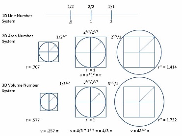 Figure 1.
Note that the graphic of figure 1 does not illustrate the 1D linear number system in Larson’s cube, as it does the 2D and 3D systems. This is because I did not understand at the time I first made the graphic that, just as our RSt here at the LRC differs from Larson’s RSt, in that it BEGINS with 3D entities, the 3D oscillations of SUDRs and TUDRs, rather than with the 1D entities, the 1D oscillations of photons, with which Larson’s RSt begins, so too should our new number systems.
We can do this by writing one system equation, with three values of n: n1, n2, n3, in the 3D equation of the Pathagorean theorem, as follows:
e/(1/e) = e2 = ((n12 + n22 + n32)1/2)/(1/((n12 + n22 + n32)1/2),
where n2 and n3 = 0, for the 1D system,
and n3 = 0, for the 2D system.
The result is the three progression series, 1(n2), 2(n2) and 3(n2), shown above in 1), 2) and 3), respectively, for sucessive values of n1, n2 and n3.
While this simplification of the current multi-dimensional number system that is based on imaginary numbers (i.e. the square root of -1), may not appear to be relevant, at this point, to a civilization that has managed to construct the marvels of modern science and mathematics, building upon this imaginary foundation, we must remember that the theoretical physics community cannot complete it’s explanation of reality on this basis, given that quantum mechanics and general relativity are fundamentally incompatible.
It must be recognized that the dimensions of the fundamental energy equation, E = mc2, are the dimensions of inverse motion and that it follows that this fact cannot be ignored in light of our thesis that the universe consists of nothing but motion and its inverse.
This is especially clear, given Xavier Borg’s demonstration that the true physical dimensions of all physical units are the dimensions of motion (sn/tn) and inverse motion (tn/sn), where n = 0, 1, 2 or 3. Thus, the mass energy equation can be written in terms of these dimensions of motion and its inverse,
E=mc2 =
(t/s) = (t3/s3)x(s2/t2),
and the radiation energy equation can also be written in these terms, when the frequency term is recognized as just a convenient measure of vibration, clarifying the dimensions of Planck’s constant, s2/t, the dimensions of the so-called “quantum of action,” which dimensions are simply an ad-hoc compensation, derived to compensate for the use of the non-physical, but mathematical expression of the frequency term, 1/t. Making this correction, the radiative energy equation is simplified to,
E=hv =
(t/s) = (t2/s2)x(s/t).
However, treatment of physical equations such as these, and their implications, will be handled in our New Physics blog. For our purposes here in the New Math blog, it is sufficient to reform the number systems and their associated algebras, for application to the new physics.
Trick or Truth: The Mysterious Connection Between Numbers and Motion and Geometry
Almost two years ago, now, on August 20, 2013, I wrote about a meeting I had with Bruce Peret and Gopi Krishna V, at Rainer Huck’s home. I was really happy to have had an opportunity to discuss some important ideas of the LRC’s work with these guys, but I never managed to finish the post, as my LRC work was overcome by events.
This changed, however, when I found out about a new essay contest at FQXi, and I decided to enter it, albeit in February, just before the March 4th deadline. It was very stressful, but I managed to write and submit a paper in time.
The theme of the contest is: “Trick or Truth: the Mysterious Connection Between Physics and Mathematics.” It was impossible to resist, but almost impossible to imagine that I could do justice to the theme, given the constraints FQXi puts on the essay entries and the little time that was left to write it.
Nevertheless, with much effort and prayer, I managed to meet the deadline with a paper I think made sense, even though there is nearly zero chance that it will be noticed much, with the hundreds of papers submitted, including one by Lee Smolin.
There are also typos and editing errors in it that I wish I could have discovered in time to correct. Yet, I hope that the readers there will overlook them. The effort was worthwhile, I think, because it gets the ideas of the LRC’s RSt, and thus Larson’s work, on the table of the judges, participants and readers of the essay contest, many of whom are professional mathematicians and physicists.
The title of my essay is: “Trick or Truth: The Mysterious Connection Between Numbers and Motion and Geometry.” I hope everyone will read it and comment on it at the FQXi site, when it is posted (it hasn’t appeared there yet, but should sometime next week,) but I thought I would post a corrected and expanded version of it here, as well.
And I will do that soon, but in the meantime, as a preface to the paper, I have determined to publish what I wrote nearly two years ago, after I met with Rainer, Bruce and Gopi, because, it is relevant, I think:
Yesterday I enjoyed a discussion of scalar motion fundamentals with Bruce Peret and Gopi, as we met at ISUS HQ, in SLC, UT, as guests of Rainer Huck. It was the first time that I had met Gopi, a young physics PhD student, studying in Texas, but originally from India.
It was actually a fruitful discussion, in large part due to Gopi’s interest in the LRC’s RSt, which gave me a chance to not only explain somewhat the unique development of our RSt and how it differs from Larson’s RSt, and the RS2 re-evaluation of his RSt, but also to introduce Gopi to the new ideas of scalar motion fundamentals, which we have been developing, while they have been experimenting with substituting projective geometry for Euclidean geometry in their work.
I explained how the tetraktys incapsulates the concept of two “directions” in three dimensions (four including zero), and how Larson’s 2x2x2 stack of unit cubes is the geometrical equivalent of the tetraktys, which, by adding the concept of magnitude, to the tetraktys concepts of dimension and “direction,” incapsulates the totality of scalar motion fundamentals: magnitude, dimension and “direction.”
I’m not sure how impressed he was with this phenomenal connection we have found between the binomial expansion that we call the tetraktys and the 3D stack of unit cubes we call Larson’s cube, especially in the course of the disjointed give and take of a living room discussion. However, I was so pleased with his careful and thoughtful curiosity that I entertained the idea of extending the discussion into the implications for a scalar algebra fit for use in RST theory development.
In fact, we did talk about imaginary, complex, quaternion and octonion numbers, and the algebraic pathology that the use of them engenders, but I was not able to get much beyond that except to touch briefly on Hestenes’ geometric algebra and Altmann’s paper, “Hamilton, Rodrigues, and the Quaternion Scandal.”
From there we got into quadrantal versus binary rotation, and I tried to explain how that fit into our work with 3D oscillation (“pulsation” as Gopi calls it. I like that.), and its physical explanation of the 720 degree “rotation” of the LST community’s concept of quantum spin.
I was so pumped, for having the opportunity to lay out these vital discoveries we have made here at the LRC to Bruce and Gopi, that I continued the discussion in my mind as I drove home, after our meeting had ended.
It was then I felt a great desire to finish the conversation, maybe in a message to Gopi, or a presentation at ISUS HQ, or something else. I finally settled on writing this blog entry, because it is here that we document the development process of the LRC’s efforts to develop a useful RSt.
Of course, like I said, I never actually got around to writing it then, but now I have written it for the essay contest. In fact, I wrote it three times, trying to fit it into their constraints. So, in the next few days, I will take those three versions and try to combine them into one expanded article, without the constraint of the contest rules.
Wait for it!
Update: A few days later and here is the expanded paper!
The Mathematics of Scalar Motion
In the discussion forum, there is reference to the excitement going on over at the rs2theory.org site due to the work of Miles Mathis.
Horace writes:
We have always been looking for the mathematical link between the magnitudes above and below one unit. Bruce uses the idea of projective geometry and counterspace to show how linear motion gets converted to reciprocal rotational motion below one unit (a.k.a. “crossing the unit boundary”).
It looks like Miles Mathis has found another way:
Miles Mathis wrote:
I developed an equation to find one velocity from the other, using the radius r, and I later showed that at the size of the photon, a tangential velocity of c was equivalent to an orbital velocity of 1/c.
Source: http://milesmathis.com/charge3.html
This is good news indeed for those who have accepted the departure from the fundamental postulates of Larson’s RST, but for those of us unwilling to accept the argument that requires the abandonment of Euclidean geometry in favor of projective geometry, as the geometry of the universe of motion, and a concommitant change in the wording of the second fundamental postulate, not so much.
Not that the controversial work of Miles Mathis might not be valid, it might be, but it illustrates a fundamental misunderstanding in the mathematics of scalar motion that exists in the “RS2” community.
In their “re-evaluation of the Reciprocal System of Physical Theory,” the followers of the RS2 community have accepted the notion that the inverse of translational scalar motion in the material sector of Larson’s RSt appears to be rotational motion, from the point of view of the material sector and vice-versa: The inverse of translational scalar motion in the cosmic sector appears to be rotational from the point of view of the cosmic sector.
Consequently, crossing the boundary between the two sectors involves a transition from translational c-speed to rotational 1/c-speed, which Mathis has appeared to confirm in their minds with his work differentiating orbital and tangential speeds of photons.
However, in the LRC’s view, this approach confuses the fundamental concepts of scalar motion in the universe of motion, which are based on the principle of reciprocity, easily graphed as shown below:
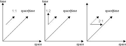
Figure 1. The Unit Boundary Between the Material and Cosmic Sectors of the Universe of Motion.
Just as 1/2 is the mathematical inverse of 2/1, Larson’s “direction” reversals in the unit space and time progression created two sectors of the universe of motion, by effectively stopping the progression of one or the other of the two reciprocal (hence orthogonal) components of the universal progression.
When the space component of an expanding location oscillates, changing the space:time progression ratio at that point from 1:1 to 1:2 (think of the increase of space as alternatingly increasing, decreasing, while the increase of time continues increasing normally), it effectively changes the progression at that point to a progression of time only, as shown in figure 1 above.
Conversly, when the time component of an expanding location oscillates, changing the space:time progression ratio at that point from 1:1 to 2:1 (think of the increase of time as alternatingly increasing, decreasing, while the increase of space continues increasing normally), it effectively changes the progression at that point to a progression of space only, as shown in figure 1 above.
This concept can be formulated mathematically by understanding that there are two interpretations of numbers: One represents quantity (how much or how many), the quantitative interpretation of number, while the other represents a relation between quantities, the operational interpretation of number.
The difference is readily understood when we consider the rational number line:
1/n, …1/3, 1/2, 1/1, 2/1, 3/1, …, n/1
The numbers to the left of unity, 1/1, are the inverse of the numbers to the right of unity. However, they may be interpreted both quantitatively and operationally, with different results, depending on the desired interpretation. Interpreted quantitatively, the numbers to the left of 1/1 are less than 1, or fractions of the whole, while the numbers to the right of 1/1 are multiples of 1.
On the other hand, interpreted operationally, the sets of numbers to the left and right of 1/1 are both multiples of 1: the set to the left are multiples of 1 in the opposite “direction” of that of the set to the right. The set to the right is the inverse of the set to the left, which changes the “direction” of its magnitudes, in the following sense:
1:n, …1:3, 1:2, 1:1, 2:1, 3:1, …, n:1
This is the sense of “direction” we have when comparing two quantities, as, for example, when we weigh quantities in a pan balance. There are three possibilites and only three: The pans are balanced with equal quantities on either side, or the pans are unbalanced with unequal quantities favoring one side or the other.
The oscillation of the space or time component at some given point in the 3D universal progression produces the discrete units of motion postulated in the first fundamental postulate of the RST. These discrete oscillating units of scalar motion may be algebraically combined and the relations between such combinations algebraically analyzed in a manner completely analogous to number systems that are well understood.
For instance, we can combine integer multiples of each:
1x(1:2) = 1:2 1x(2:1) = 2:1
2x(1:2) = 2:4 2x(2:1) = 4:2
3x(1:2) = 3:6 3x(2:1) = 6:3
. .
. .
. .
nx(1:2) = n:2n nx(2:1) = 2n:n
Clearly, in terms of magnitude and “direction,” these two sets of numbers are equivalent to opposites
-1, +1
-2, +2
-3, +3
.
.
.
-n, +n,
when quantitatively interpreted, but when operationally interpreted, they are multiplicative inverses, such that 1/n times n/1 = n/n, or unity.
When used to formulate speeds of the universe of motion, as we have illustrated in figure 1 above, we must make a distinction between material sector speeds and cosmic sector speeds, because one is speed-displacement from c-speed in terms of time, while the other is speed-displacement from c-speed in terms of space:
Material Sector Cosmic Sector
Δs/Δt = 1/1 = c Δt/Δs = 1/1 = c
Δs/Δt = 1/2 = 1Mc Δt/Δs = 1/2 = 1Cc
Δs/Δt = 2/4 = 2Mc Δt/Δs = 2/4 = 2Cc
. .
. .
. .
Δs/Δt = n/2n = nMc Δt/Δs = n/2n = nCc
Where Mc = material speed-displacement = Cc = cosmic speed-displacement = 0.5c.
Of course, because these speeds are inverses, one is four times greater than the other, quantitatively, when considered from the reciprocal point of view (i.e. 2/1 = 4x0.5).
The attempt to quantify the RST concepts has led to different approaches, but the LRC was established to ensure that Larson’s fundamental postulates were not changed in the process. Opponents object to Larson’s idea of “direction” reversals and have sought to find an alternate way to obtain the required reciprocity of the system, by resorting to rotation. This is understandable, but the LRC takes exception to the concept of rotation as scalar motion.
Of course, the rejection of rotation as scalar motion means that the LRC departs from Larson’s development of the consequences of the RST in his RSt, but it does not imply departure from the RST itself, which must be held inviolate.
In its abandonment of the RST, it appears to us that the RS2 community has lost sight of the meaning of true reciprocity and in the attempt to justify its rationale, it now seems willing even to abandon the concept of scalar motion.
Seeking Closure
Closure is something we all seek. Mathematically, it’s vital in order to successfully operate with numbers; i.e. to add, subtract and multiply and divide them consistently. Because the integers are closed under these mathematical operations, so too are the non-zero rationals.
However, the integer and rational number systems are actually composed of one dimensional numbers, or lengths. As we have discussed many times before, to deal with higher dimensional numbers, legacy system mathematics adds “imaginary” numbers to these number systems.
In the reciprocal system of mathematics (RSM), we recognize four scalar dimensions, with two “directions” each. At unit magnitude, these are isomorphic to the 4th degree of the binomial expansion, 20, 21, 22 and 23, which we call the tetraktys, because it consists of the first four numbers of the Pythagorean system of numbers: the monad, the dyad, the triad and the tetrad.
As we happily discovered some time ago, the binomial expansion of the tetraktys is the numerical equivalent of the geometry of the 2x2x2 stack of 8 unit cubes that we call Larson’s cube (LC). Its center, located where one corner of all 8 cubes coincide, defines the middle point of three, 1D, orthogonal lines, the intersection of three, 2D, orthogonal planes, as well as the intersection of the diagonals drawn between the eight reciprocal corners of the stack.
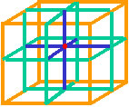
Figure 1. The Stack of Eight 1-unit Cubes Known as Larson’s Cube
The fact that this geometric figure contains the geometric representation of the four dimensions of the tetraktys and thus the first four binomial expansions of the tetraktys (counting zero), it follows that it also connects geometry with the eight mathematical dimensions of the four normed division algebras, the positive and negative reals, complexes, quaternions and octonions.
Moreover, the geometry of the LC not only represents the numbers of the tetraktys, it also defines a unit volume within its interior, and defines the inverse of this volume with its extent, a fact that connects the integer and rational numbers with irrational numbers, in a fundamental manner.
This connection between integers, rationals and irrationals provides a different approach to numbers and number systems that is not defined by Cantor’s sets nor Dedekind’s cuts, nor imaginary numbers. It is based on scalar expansion, where the three 1D lines, the three 2D planes and the eight 3D cubes expand outward from the 0D point.
Since a unit of space and a unit of time can be defined for the LC expansion, from point to cube, it follows that a unit of motion, v = Δs/Δt, can also be defined for it, and the inverse of the outward expansion, the unit inward motion of collapse. Since such a motion has only two possibilities, outward or inward, we can define them as the two scalar “directions” of motion, in contrast to the possible vector motion directions, which is a set of infinite directions.
Because these two scalar “directions” of motion, outward and inward, manifest themselves in each of the non-zero geometric components of the LC (the 1D line, the 2D area, the 3D volume), it’s easy to confuse them with the geometric “directions,” or poles associated with each of these entities, but we should note that the two poles of the 1D line can expand and contract, the four poles of the 2D area can expand and contract and the eight poles of the 3D volume can expand and contract.
Hence, we can use the base number 2 with non-zero exponents 1, 2 and 3 to represent the total “directions” of each non-zero dimension’s expansion, as indicated by the exponents: 21 = 2; 22 = 4, 23 = 8 “directions” respectively.
Given this isomorphism between the magnitude, dimension and “direction” of geometric expansion of the LC, and the magnitude, dimension and “direction” of the numerical expansion of the tetraktys, the question arises, “Can these geometric and numerical entities be used to form a number system that is closed under addition, subtraction, multiplication and division?” If the answer is “yes,” then it follows that the resulting 3D algebra will also have 2D, 1D, and 0D subalgebras that are closed as well.
While this may seem obvious given Clifford algebras, it isn’t, because the dimensions of the 3D Clifford algebra are used only to define the 1D (vector) space that the Clifford algebra operates in. Thus, it is all about the mathematical operations that translate and rotate vectors in that space.
In our case, we are dealing with an algebra of the spaces themselves. We seek to add and multiply LCs, if you will - the whole LC at once, represented by its geometric properties and the isomorphic numerical properties of the tetraktys.
As described in the previous entry, the numerical expansion of the LC, and thus the tetraktys, can be accomplished by addition or multiplication of its poles. Since the monopole, the three dipoles, the three quadrupoles and the single octopole comprise the unit and its subunits, they can be consistently manipulated algebraically.
To demonstrate this requires only that the geometric coefficients (1331) of the four-part numbers (1(20)+3(21)+3(22)+1(23)) be removed, before the algebraic operation is performed, and then reinserted into the number after the calculation is complete. For example, we can show that this works for addition, subtraction, multiplication and division, by letting the unit LC equal ‘a.’ Then,
a = (1+2+4+8)
b = 2a = 2 x (1+2+4+8) = (2+4+8+16)
c = 3a = 3 x (1+2+4+8) = (3+6+12+24)
d = 4a = 4 x (1+2+4+8) = (4+8+16+32)
Next we perform the following operations:
For multiplication,
1) a/b x c/d = ac/bd
((1+2+4+8)/(2+4+8+16)) x ((3+6+12+24)/(4+8+16+32)) =
((1+2+4+8)(3+6+12+24)/((2+4+8+16)(4+8+16+32)) =
((3+12+48+192)/(8+32+128+512)) =
((3(1+4+16+64))/(8(1+4+16+64)) = 3(1+2+4+8)2/8(1+2+4+8)2 = 3/8
Just as a/2a x 3a/4a = a(3a)/(2a)(4a) = (3a2)/(8a2) = 3/8
For addition,
2) a/b+c/d = ad+bc/bd =
(1+2+4+8)/(2+4+8+16) + (3+6+12+24)/(4+8+16+32) =
((1+2+4+8)(4+8+16+32) + (2+4+8+16)(3+6+12+24))/((2+4+8+16)(4+8+16+32)) =
((4+16+64+256)+(6+24+96+384))/(8+32+128+512) =
(10+40+160+640)/(8+32+128+512) =
10(1+4+16+64)/8(1+4+16+64) =
10(1+2+4+8)2/8(1+2+4+8)2 = 5/4
Just as
(a/2a)+(3a/4a) = ((a x 4a)+(2a x 3a))/(2a x 4a) = 10a2/8a2 = 10/8 = 5/4
And finally, for division,
3) (a/b)/(c/d) = (ad)/(bc) =
((1+2+4+8)/(2+4+8+16))/((3+6+12+24)/(4+8+16+32)) =
((1+2+4+8)(4+8+16+32))/((2+4+8+16)(3+6+12+24)] =
(4+16+64+256)/(6+24+96+384) =
4(1+4+16+64)/6(1+4+16+64) = 4(1+2+4+8)2/6(1+2+4+8)2 = 2/3
Just as
(a/2a)/(3a/4a) = (a(4a))/((2a)(3a)) = (4a2)/(6a2) = 2/3
Of course, since a = 1, 2/3 = 2a/3a = 2(1+2+4+8)/3(1+2+4+8) or, equivalently, 2(20+21+22+23)/3(20+21+22+23)
With the calculation complete, we insert the geometric numbers (1331) back into the final terms, which gives us the correct number of poles. For instance, in this last example,
2(20+3(21)+3(22)+23) = (2+12+24+16) = 54
3(20+3(21)+3(22)+23) = (3+18+36+24) = 81
54/81 = 2/3.
But then, why not just use the number of poles in the LC to begin with?
LCp = (1x(20)+3x(21)+3x(22)+1x(23)) = (1+6+12+8) = 27,
and since 27 = 33, then let
a = 33
b = 2(33)
c = 3(33)
d = 4(33)
and naturally, the algebra is still closed under addition and multiplication.