The Larson Research Center

The Structure of the Physical Universe

Combinations <<<———->>>>> Dimensions

Material Sector Magnitudes

1. M_g = balanced RN
2. M_r = SUDR imbalance
3. M_b = TUDR imbalance

and the notation for the Cosmic sector dimensions (time/space) is,

1. C_g = balanced RN
2. C_r = TUDR imbalance
3. C_b = SUDR imbalance

However, the magnitude of all vectors of the VT, in both GA and vector algebra, is obtained by scalar multiplication, even though, in GA, the scalar is regarded as the zero grade blade occupying its own vector space. Again, this contrast with vector algebra, where the vector space of the higher dimensional vector is obtained by the introduction of ad hoc imaginary numbers and combining these with the 2⁰ real numbers to form the 2¹ complex numbers of the plane. This means that vector algebra operates in the two spaces of the complexes, where the scalar magnitudes of real numbers can be defined in any direction in the complex plane defined by a complex number. Thus, using the inner and cross vector product, vector algebra can operate on the radius vector contained in a sphere of any magnitude in any direction from the origin.

Modern science and technology are based on the concepts of vector algebra, operating on line two of the VT (the complexes). Yet, intuitively, one would think that GA, operating on line four of the VT (the octonions), would be much more powerful, since its operations have a much more complete correspondence to Euclidean geometry. However, while the greater power of GA is being recognized more and more today, many scientists, familiar with vector algebra and its many successes, are not easily convinced that GA is necessarily more useful than vector algebra. Nevertheless, this preference for vector algebra is destined to eventually die out, as surely as the early preference for the analog slide rule over the digital computer eventually died out.

As computer technology matured, the power of its more fundamental digital abstraction could be exploited more and more efficiently, first in mainframe computers, and then in electronic calculators and personal computers, until its superiority was clearly manifest, leading the community of scientists and engineers to abandon the analog-based slide-rule altogether. Similarly, the more fundamental abstraction of GA is not yet fully exploited, but as more and more ways are found to take advantage of it, ways not foreseen in the beginning, any more than the myriad ways to use digital technology were foreseen, the use of GA will become ubiquitous.

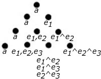
One of the most important unforeseen applications of GA is its use in understanding level four of the VT in terms of its four vector spaces (2⁰, 2¹, 2², 2³). As explained in the Dimensions section of the SPUD, these four vector spaces correspond to four scalar spaces in the Scalar Tetraktys (ST.) The correspondence is dramatically demonstrated in figure 1 below:

When we compare the use of vector algebra in LST physics, to the use of GA in LST physics, the performance of the two algebras is best understood in terms of describing vectors as rotations. To describe rotations with vector algebra is like constructing a building with one-dimensional lumber, where walls are first constructed by nailing studs together and then covering them with two-dimensional dry-wall material. In contrast, using GA, the material comes as one, two, and three-dimensional material, so that walls and rooms don’t have to be constructed from one-dimensional objects first.

However, in most applications of LST physics, motion is always one-dimensional, and, so, even though the rotation of one-dimensional motion is more easily described in the language of GA, it is still one-dimensional magnitude, represented by a vector, and whether the operation of that vector magnitude, with a second vector magnitude, is calculated as a resultant vector, a normal vector, or a scalar magnitude, using vector algebra, or as the rotation of a bivector, using GA, does not make much difference in the final analysis. Hence, the advantage of GA is not all that apparent in these applications.

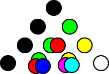
Nevertheless, in RST physics we are not limited to the one-dimensional motion of the LST. In the RST, magnitudes of motion consists of one, two, and three-dimensional ratios of space and time, and since these scalar ratios are themselves scalar values, we can represent them with the scalar values of color, as shown in figure 1 above, where each of three, orthogonal, values (red, green, and blue) is the result of the dimensional expansion of the scalar, represented as the color black, in three dimensions.

Combining two of these scalar values, from the one-grade scalar space, produces a new scalar value in the two-grade scalar space, just as combining two vector values, from the one-grade vector space, produces a new vector value in the two-grade vector space. However, whereas it is direction that defines the orthogonality of three vectors, and thus provides a “basis” for the calculation of magnitude in any direction in 3D vector space, a sphere, it is “direction” that defines the orthogonality of three scalars, and thus provides the basis for the calculation of magnitude in any “direction” in 3D scalar space, a “volume” consisting of three colors.

Using colors as analogs for scalar motion, we see that the color black (lack of color) is the inverse of white (all colors), just as the geometric point (lack of “direction”) is the inverse of the geometric volume (all “directions”). Moreover, all colors can be subdivided into all two-dimensional colors, or all one-dimensional colors, with respect to the color black (origin of the color white, or “volume”), just as the geometric volume can be subdivided into all two-dimensional directions (planes), or all one-dimensional directions (lines) with respect to the geometric point (origin of the spatial volume).

Of course, since there is a one-to-one correspondence between the scalar color combinations of line four of the ST, and the scalar motion combinations of M_g, M_r, and M_b, we can see that colors may be “painted” to depict the magnitudes of n-dimensional scalar values of the ST, just as lines may be drawn to depict n-dimensional vector values of the VT.

Furthermore, we can see that the “orthogonality” of the three primary colors, red, green, and blue, permit us to use them as the basis set for the one-grade space of the ST, just as the orthogonality of three intersecting lines permit them to be used as the basis set for the one-grade space of the VT.

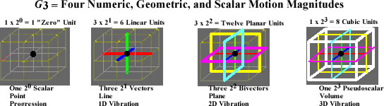
Visualizing the VT in Larson’s Cube, we can see how each of its four vector spaces relate to each other. Indeed, these spaces are well defined by scalar vibrations, where the vibrations are defined as a unit expanding/contracting point in three dimensions. A basis for calculating all one, two, and three-dimensional magnitudes, are formed by the three orthogonal lines, and the three orthogonal planes, intersecting at the point, as shown in figure 2 below.

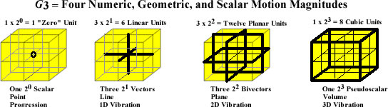
In the case of scalar vibrations, the point at the far left becomes the volume at the far right, over time. Hence, if, at time t₀, the geometry of the scalar magnitude is a point, and at time t₁, it expands to a volume, then at time t₂ it contracts to a point again, the scalar expansion of the scalar point to the pseudoscalar volume, expands all the one-dimensional lines, and all the two-dimensional planes in the volume, as well.

In other words, using the three orthogonal lines and the three orthogonal planes as a basis set in their respective scalar spaces, the expansion of the scalar point can be expressed as an expansion of any 1D line in the volume, or as any 2D plane in the volume, from the scalar point, at t₀, to a 1D line, or a 2D plane, at t₁, and back to the scalar point at t₂.

The scalar vibrational motion thus described, is the scalar motion of the SUDR, when the geometry is spatial, and the scalar motion of the TUDR, when the geometry is temporal (in the Cosmic sector). These two geometries (spatial and temporal) are combined in the SUDR|TUDR combo, as depicted in the world line chart of figure 2 of the previous Dimension section of the SPUD. As explained in that section, the SUDRs of the Material sector, and the TUDRs of the Cosmic sector, can combine to form a SUDR|TUDR combo (S|T unit) that has components in both sectors. The initial combo is the first RN of the RSM, or M_g in the notation introduced above.

The scalar “orthogonality” is in scalar “directions,” not spatial directions; that is, we can have “green” magnitude, or “red” magnitude, or “blue” magnitude, and combinations of these “orthogonal” color magnitudes, gives us new color magnitudes, representing the “orthogonal” relationship between them. The scalar “orthogonal” relationship is depicted in figure 4 below, as a spatial orthogonal relationship. The important point to grasp is that the right angles in the illustrations are a convenient, not a necessary, configuration of the scalar “orthogonality;” that is, the result of the color mixing does not depend on the depicted angle, any more than the result of mixing colors of paint depends on the relative locations of buckets of paint.

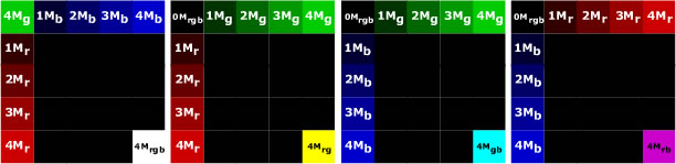
The second graphic from the left is the first graphic rotated ninety degrees to the right so that the blue axis is rotated out of the plane of the page. The upper left square of the first graphic shows the top of the green magnitudes (4M_g), while the upper left square of the second graphic shows the bottom of all the magnitudes, which is the black scalar (1/1 = no color) of the UPR, or the infinite void, which is the origin of all the ST spaces. It is the zero-grade scalar space, corresponding to the zero-grade point in figure 2.

The third graphic from the left rotates the second graphic’s column of red magnitudes to the vertical position, rotating the blue magnitudes back into the plane of the page, from out of the plane of the page. However, the red magnitudes are collapsed to zero, in order to show the 2D 4(green-blue) combo, instead of the 4(red-green-blue), or white, combo of the first graphic.

The fourth graphic from the left rotates the third graphic’s column of green magnitudes out of the plane of the page, giving us a view of the bottom of the green column once again and expanding the red column to full value. Clearly, the yellow, cyan, and magenta colors of the bottom right squares of the three graphics to the right of the first graphic, are the three basis colors of the 2D scalar space, while the 4(red-green-blue), or white, color of the bottom right square of the first graphic, is the one basis color of the 3D scalar space.

This definitely shows that the analog of the scalar motion, the scalar colors, and the vectorial spaces defined by vibrational scalar motion, are isomorphic; that is, the 1D, 2D, and 3D scalar values of the ST are isomorphic (isometric?) to the vector values of the VT, in that n-dimensional scalar magnitudes can be formed algebraically, as combinations of the basis values. In other words, the familiar use of RGB color mixing, to produce the full range of colors, is tantamount to using the RNs, to produce the full range of 0D, 1D, 2D, and 3D magnitudes of the ST.

Hence, we conclude that (aMr + bMg + cMb), as a measure of the scalar magnitude of three scalar dimensions, is just as much a three-dimensional scalar magnitude in the ST, as (ae₁ ^ be₂ ^ ce₃), as a measure of the geometric magnitude in three geometric dimensions, is a three-dimensional geometric magnitude in the VT. The difference in the algebra of the two kinds of numbers is that the algebra of the ST is ordered, commutative, and associative over addition and multiplication, whereas the algebra of the VT is not necessarily. In the VT, the bivector and trivector are not commutative.  Figure 5 illustrates the ST-VT correspondence.