The Larson Research Center

Larson wrote a book entitled Beyond Newton, and people now days talk about physics “beyond the standard model,” but the standard model is really the crowning achievement of Newton’s program, and to go beyond Newton is to go beyond the standard model. 

However, Larson never really compared his work with the standard model in any direct way.  He wrote his Case Against the Nuclear Atom, but this was early on.  By the time the standard model was in place in the late seventies and became  somewhat accessible to non-professionals in the eighties, it was too late.  The members of ISUS not only were never able to address the standard model viz-a-viz the RST, but they generally took an attitude of animosity towards it and the quantum mechanics it rode in on.

Nevertheless, it is embarrassing that, while the standard model is capable of very accurately predicting the fundamental interactions among the debris of high energy particle collisions in the accelerators, Larson’s physical theory, the RSt, which he developed from the new system of physical theory, the RST, can not even play in that game. It’s as if the standard model could predict where every ball ends up, from the opening break on a pool table, but while the RSt has nothing to say about the positions of the balls, it can tell us what the standard model cannot tell us - what the balls on the pool table are made of. 

Hence, both the standard model and the RSt are incomplete.  Newton’s program assumes the existence of matter, radiation, and energy, with the properties of propagation, gravitation, mass, charge, spin, etc. as inputs (19 - 24 such parameters altogether) to the standard model, but has worked out the “fundamental” interactions of matter in terms of M2 motion.  The RSt, on the other hand, assumes only the existence of M4 motion, with its properties of quantum units and two reciprocal aspects, but has worked out the fundamental composition of matter, radiation, and energy, with their respective properties, in terms of M4.

The reason why I place quotes around “fundamental” in the phrase “fundamental” interactions is that this indicates the source of the aforementioned animosity among ISUS members towards the standard model.  Force, Larson argued, is a property of motion, by definition, and cannot exist as an autonomous, or “fundamental,” entity. The fact that the LST community has ignored this implication of the definition of force is one of the major Neglected Facts of Science, Larson wrote about so compellingly.

However, this temptation to smugness is something that members of the Society cannot afford to indulge, as honest investigators of the truth.  The standard model is not regarded as the greatest intellectual achievement of the 20th Century for nothing.  The modern world of high-energy physics, and physics in general, depends upon the understanding inherent in it.  How foolish do we look, if we deny its worth, just because we think we know that forces can’t be fundamental?

What we really need to do is to roll up our sleeves and go to work to find the common ground between the standard model and the RSt.  To do this, we need, first of all, to understand what the standard model of “fundamental” forces is and how it works, so that we can relate its concepts and principles to those of the RSt.  Of course, here at the LRC, since we are developing the RSt along somewhat different lines than Larson did, the challenge is to relate the standard model to our particular development, which we are documenting in the SPUD. 

In the SPUD, we show how the “direction” reversals in the unit progression, shown in the PAs, lead to the formation of reciprocal, unit, speed-displacements, called SUDRs and TUDRs.  We show how these discrete units of space/time progression, located on either side of the unit space/time progression line, in our  world line charts, and their combination, as S|T combos, located on the unit progression line of the charts, relate to the space/time progression in general.  However, we can further clarify what the S|T combination entails by incorporating the motion of the PAs on the charts, as shown in figure 1 below:

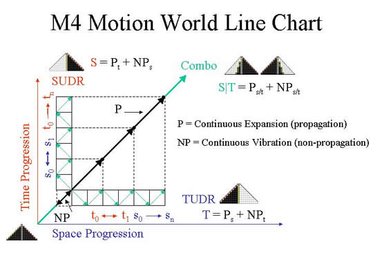
Figure 1.  M4 (scalar) Motion World Line Chart

Figure 1 shows that M4 motion consists of two motions simultaneously.  The propagation motion of continual s/t increase, and the non-propagation motion of continual s/t increase/decrease, are both components of the S|T combo.  What this means, in effect, is that the S|T combo is both a point and a pseudopoint, simultaneously.  Of course, the pseudopoint is a 3D expansion, while the point is a 3D oscillation, so the coordinates of the chart are points in the sense of the value q, specified by three coordinate points. Thus, a change in q indicates a change in volume, or size.  Red ques (red s) are space coordinates, while blue ques (blue t) are time coordinates. 

The 3D expansion, or pseudopoint (P), continues expanding, as long as space and time are progressing, but the 3D point associated with it, and inseparably connected to it (NP), remains stationary in the space/time location of its origination, unless acted upon by an outside agency.  However, since the frequency of the TUDR (2) is four times higher than the frequency of the SUDR (.5), from the perspective of the SUDR space/time location, the natural harmonics are present as well; that is, a frequency twice that of the SUDR (the first octave from the fundamental SUDR frequency and the second harmonic), three times it (third harmonic), and four times it (fourth harmonic and second octave, the TUDR). These harmonics play a significant role in the structure of the S|T combo, but I won’t comment on this aspect for now.

What I want to point out now is that since the S|T entity consists of two types of M4 motion, the continual expansion and the continual oscillation, as clearly show in figure 1, there are two ways that it can interact with other, similar, entities: one way is as a stationary entity of unit size, and the other is as an expanding entity of unit speed.  As the chart in figure 1 shows, the first is a 1/1 ratio, while the other is a 2/2 ratio, but this is deceiving, because the oscillation of the NP motion, as indicated by the double-headed arrow in the lower left box, hides the fact that it is also two units of motion, one each in two “directions.”  Thus, the total motion is actually P + NP = 2/2 + 2/2 = 4/4 units of M4 motion, which is what the RN equation expresses (ds/dt = 1/2 + 1/1 + 2/1 = 4/4).

In the SPUD, we show how adding M4 units of SUDR or TUDR motion to the S|T combo, balances it, or unbalances it, but in all cases the total number of units is always a unit value, n/n.  This aggregation-of-units process increases the quantity of the units in the combo, or its density of space/time we might say.  However, it also shows how this system of motion must relate to the standard model on a fundamental level.  We reach this conclusion based on the following considerations:

The fundamental classification of the standard model classifies physical entities in terms of three interactions:

1. The “strong force” that forms heavy units of matter called hadrons (e.g. protons and neutrons).
2. The “weak force” that binds these units of matter together into nucleons of hadrons.
3. The “electromagnetic force” that binds lighter units of matter called leptons to the nucleons made up of hadrons, to form atomic units.

In the tetraktys of motion, containing the four bases of motion, we have the same classification, but in terms of motion, not forces:

1. M4 motion, which is motion, based on change of scale (numbers) in the bound units (SUDRs & TUDRs bound as S|T units).
2. M2 motion, which is motion, based on change of position between bound, or S|T, units of M4 motion.
3. M3 motion, which is motion, based on an internal, change of interval, motion in the oscillation component of the M4 bound units.

Of course, this is just a start, but already the parallels are striking.  The S|T units may be balanced or unbalanced.  If unbalanced, the unbalance is in two, opposite “directions,” giving us three possibilities that are parallel to the three possibilities of the standard model: neutral, positive, or negative.  The neutral, positive, and negative values come in discrete values.  The lighter values of neutral, positive and negative are much lighter than the heavier values of neutral, positive and negative, but the scalar difference is not in the “density” of the “directions,” neutral, positive, or negative, but in the magnitude of the total density; that is, a much heavier neutral entity, can be unbalanced, or “charged,” by just one unit of “direction,”  in the same manner, and to the same magnitude, as the lighter neutral entities.

We’ve been aware of the “direction” parallel for some time now, but the concept of the two simultaneous components of M4 entities is new, and the parallel with the standard model that we see right off is in the de Broglie relation, where each quantum physical entity has an associated wavelength, given by:

λ = h/ρ

where h is Planck’s constant and p is the momentum of the entity.  If Planck’s constant is proportional to P in M4 and its “momentum” is proportional to the NP component, then what we have is the same ratio; that is, the wavelength, s, is just an expression of the unit ratio of P/NP = (2/2)/(2/2) = 1, or the ratio of the two components of the natural unit of motion, 4/4 = 1/1.  To see this, we have to recall Larson’s insistence that the dimensions of h are t²/s², the same as momentum, not the dimensions of action, t²/s.  Thus, if Larson is correct, we get

(t²/s²)/(t²/s²)  = 1, not s.

Hence, we conclude that the de Broglie relation is part of the RST model, as well as the standard model.  There are many other parallels, which we will be pointing out as we approach the answer to the question, “What is conserved in the transformation of M4 motion?” but that’s enough for now.