In the comments section, there’s been discussion about employing the wave equation in our research, expanding our outreach efforts and taking note of the work of Miles Mathis. In each case, I felt the resistance of initial inertia, but eventually began to experience some momentum building in my thoughts and feelings about these things.
Our immediate research goal here at the LRC is to arrive at the point where we can calculate the atomic spectra, using our RST-based theory (our RSt). The LST community’s ability to do this (well, in principle, anyway) and our inability to do it is embarassing. Nehru called it the “glaring lacuna” of Larson’s RSt (see here.)
While pursuing this goal, we’ve discovered many wonderful things, but none of them has enabled us to do the calculations yet. Perhaps, we may be finding ourselves agreeing with Nehru that the use of the wave equation may be inevitable after all, if we are going to reach our goal.
However, there are some intriguing conceptual developments that are closely related to the atomic spectra, which show the fundamental difference between the LST and the RST that has to be taken into account, if we are to use the wave equation in our calculations. The LST defines motion as a change in an object’s location, the distance between locations over the time it takes to travel that distance.
This idea of translational motion is extended to rotation, but the “distance” traveled is measured in terms of a time rate of change in the quantity of radians, or unit angles. We can count between the cardinal points on a circle, in terms of π:
t0…………t1…………t2………….t3…………..t4
0………(π/2)……….(2π/2)……….(3π/2)………(4π/2)
But when this convention was employed in quantum physics to describe quantum spin, it was found necessary to modify it to:
0……..(π/2)………(2π/2)………(3π/2)……..(4π/2)……..(5π/2)………(6π/2)………(7π/2)………(8π/2),
because one revolution of quantum spin requires twice as much rotation as one revolution of non-quantum spin, something not understood to this day in the LST community.
Since the LST concept of quantum spin, as incomprehensible as it is, was the key to the breakthrough of quantum physics in the LST community and its successful calculation of atomic spectra energy levels, it’s important to understand how it relates to the RST theory of atomic spectra energy levels, which has no concept of spinning electrons, whirling around a nucleus of protons and neutrons.
Moreover, in our LRC RSt, unlike in Larson’s RSt, and in Nehru’s modification of Larson’s RSt, there is no concept of rotation! Nehru sought to employ complex numbers to represent what he called “one-dimensional spin” in the time (inverse) region of the universe of motion, because time is 3D in this region and space is scalar. He also extended this approach to the use of quaternions to represent what he called “two-dimensional spin.” The 1D spin applies to what Nehru called the “Atomic Zone,” while the 2D spin applies to what he called the “Nuclear Zone.”
These time region studies see a 1D “electronic” potential between rotation in the complex plane and the 3D unit progression, and a 2D “nuclear” potential between the rotation of the 1D rotation itself in an orthogonal dimension and the universal progression. The former, is formulated in terms of 2D complex numbers, while the latter is formulated in terms of 4D quaternions. This follows pretty much the LST approach to calculating these potentials with Lie algebras, but replaces the LST concepts of the atom, such as electron clouds and nuclei, with RSt concepts of n-dimensional scalar rotations, forming the atoms, which oppose the universal expansion.
However, since the LRC RSt concept requires an initial 3D oscillation of the space (time) aspect of the progression, with compounds of the resulting entities forming the bosons and fermions of the universe of motion, we must find the corresponding “electronic” and “nuclear” potentials in these 3D entities, without recourse to n-dimensional “scalar rotations.”
Apparently, the way to proceed in our case is to extend the idea of Larson’s 1D scalar speed-displacements in a natural way, which we have tried our best to do, by first understanding the mathematics of scalar motion, which is manifestly different than that of vector motion. Three-dimensional scalar motion does not involve the changing location of an object, but the changing size of an oscillating volume.
This periodic change in volume occurs from postulated changes in the outward “direction” of the universal space/time expansion, at a given point in that expansion. We can express the unit 3D expansion in algebraic terms, by expanding Larson’s cube (LC) over time:
t0…………t1…………t2………….t3…………..t4
10…………23………..43………….63………….83
But the 3D ocillation, reversing at each unit, introduces a differential between it and the progression, which is determined by a given dimension of the oscillation. For its 1D component, for example, the 3D scalar expansion is:
11…………21………….41………….61………….81,
creating the unit speed-displacement in one dimension:
10…………out:21/(out:1x21)………..out:41/(in:2x21)………….out:61/(out:3x21)………….out:81/(in:4x21),
or a 1D unit speed-displacement: 1:2.
However, for the 2D component of the 3D scalar expansion, we get:
10…………22………..42………….62………….82,
creating a unit speed-displacement in two dimensions:
10…………22/(1x22)………..42/(2x22)………….62/(3x22)………….82/(4x22),
or a 2D unit speed-displacement:12:22.
For the 3D component of the scalar expansion, we get:
10…………23………..43………….63………….83,
creating a unit speed-displacement in three dimensions:
10…………23/(1x23)………..43/(2x23)………….63/(3x23)………….83/(4x23),
or a 3D unit speed-displacement:13:23.
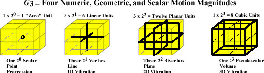
This shows we’re in the game and what’s more, the discovery of Miles Mathis that π = 4, in kinematic equations, places the 3D potential squarely in our Wheel of Motion, as each group of elements follows a 4n2 , or a πn2 relation.
But we need to quantify the physical expansion/contraction using continuous magnitudes, since nature doesn’t expand by cubes. One way to do this is to divide the volume of the unit ball into 8 sub-unit balls that have a volume corresponding to the 8 1-unit cubes in the 23 stack of unit cubes of the LC.
The volume of the unit ball is just 4π/3, since r = 1. Thus, (4π/3)/8 is the sub-unit volume we need, and, as it turns out, the radius of this 1/8 volume is just the cube root of its ratio to the unit volume, or the cube root of 1/8, which is 1/2.
V1 = (4π/3), V2 = V1/8
V2 = (4π/3)r3
r3 = (V2/V1) = 1/8
r = (1/8)1/3 = .5
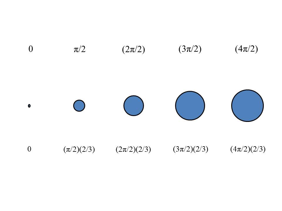
Now, if we map these sub-unit volumes (SV) to angles of rotation of the unit circle, we can construct a rotational analog of the volume oscillation. Our first four points of reference on the unit circle for the first four volumes are:
SV0…..SV1…..SV2…..SV3……SV4.
and our first four angles of rotation are:
0………(π/2)……….(2π/2)……….(3π/2)……….(4π/2),
Happily, 1/8th of the unit volume is equal to (π/2)/3, so our 3D scalar to 2D rotation map is:
0…..(π/2)(2/3)……(2π/2)(2/3)…..(3π/2)(2/3)…..(4π/2)(2/3)
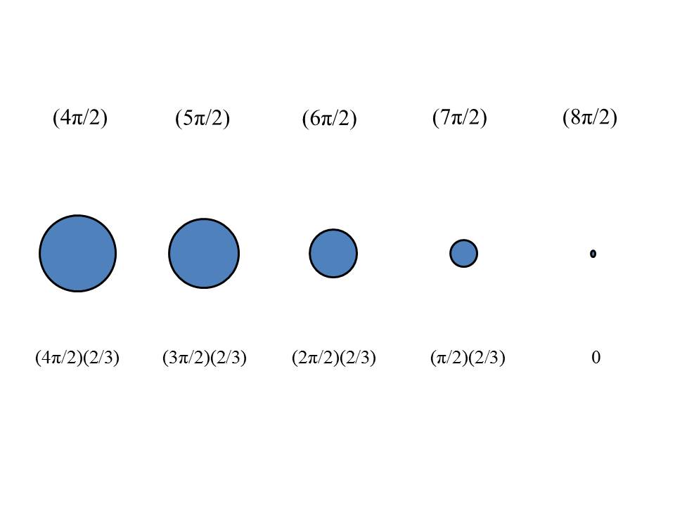
which fills from 0 to unit volume in 1 unit of time, the expansion, and then the contraction deflates, from unit volume back to the starting point (0), taking another unit of time:
(4π/2)………(5π/2)……….(6π/2)……….(7π/2)……….(8π/2),
(4π/2)(2/3)…..(3π/2)(2/3)……(2π/2)(2/3)……..(π/2)(2/3)……….0
This is a significant achievement of the RST. Bruce Schaumm, on page 187 of his book, Deep Down Things, linked above, writes:
We don’t really have a clue about the physical origin of [quantum] spin. To describe spin as “intrinsic angular momentum” is like your best buddy describing how your car’s differential works by explaining that it “employs a mechanical linkage;” the only useful information contained in this statement is that its author probably knows next to nothing about how a differential actually works.
Well, it’s not all that hard to explain in the universe of motion:
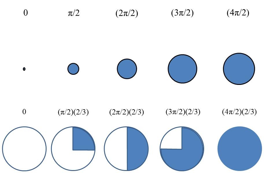
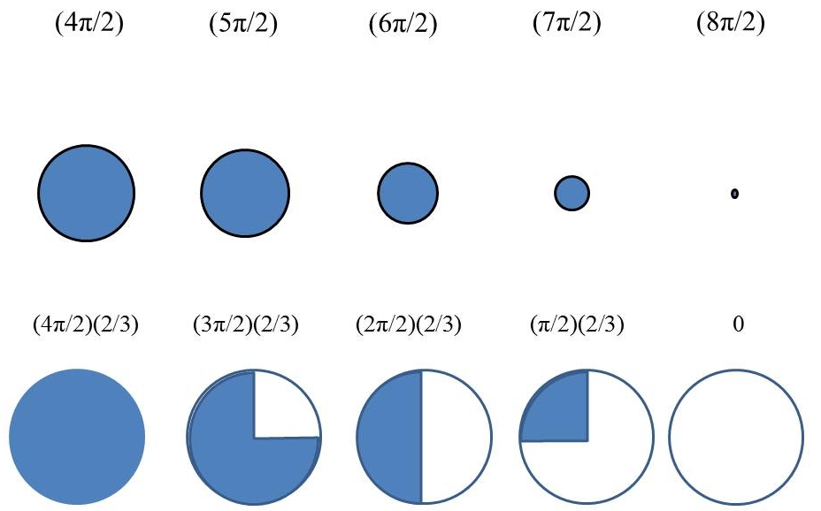
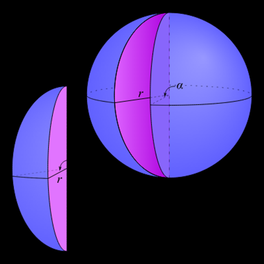
The reason it seems that it takes two 2π revolutions to complete one cycle of quantum spin is that the “spin” is not actually 1D rotation, in 2D space, but the 3D oscillation of a volume in 3D space, as depicted below:
In the equivalent of one revolution of 2π, the 3D oscillation has fully expanded, which is one-half of its cycle. To return to the starting point at zero, requires a second unit of time, and the equivalent of a second 2π revolution. With this map of 3D oscillation to 2D rotation, we ought to be able to adapt the wave equation to move forward in the goal to calculate the atomic spectra.
UPDATE: As (π/2)/3 = .523598… = V1/8, two of these volumes, or V = (π/2)(2/3), are the equivalent of one π/2 rotation (90o.)
2nd Update: The above update is in error, since (π/2)/3 = .523598… radians = V1/8 = 30 degrees, not 45 degrees. Hence, the calculations shown are incorrect. The correct calculations are shown below:
If we map these 8 sub-unit volumes (SV) to 4, 90, degree segments of 2π rotation of the unit circle, we can construct a rotational analog of the volume oscillation. Our first 4 points of 90 degree reference on the unit circle for the first 4 sub volumes are:
SV0…..SV1…..SV2…..SV3……SV4
and our first 4 segments of 90 degree equivalent rotation are:
0………(π/2)……….(2(π/2))……….(3(π/2))……….(4(π/2)),
Mapping the 1/4 volume to π/2 radian of rotation, the required delta in volume per 90 degrees of rotation, gives us .66667 volume units per 90 degrees of rotation:
V/x = π/2
x/V = 2/π
x = V(2/π)
x = 2.6666,
V/x = 4.18879/2.66667 = .66667 volume units, per 90 degrees of rotation.
Hence, the value of the 8 SVs in the original calculation does not correspond to the four, 90 degree rotations, as indicated in the graphic. In terms of radians, each of the 8 SVs is equivalent to 30 degrees of rotation, not 90.
Therefore, each delta in volume, corresponding to 90 degrees of rotation has nothing to do with the eight sub-volumes in the LC.
Instead,
0……..(π/2)………..(2(π/2))……….(3(π/2))……….(4(π/2)) =
0…..(.66667)…..(2(.66667))…..(3(.66667))…..(4(.66667)),
which fills the volume from 0 to unit volume in 1 unit of time, the expansion, and then the contraction deflates, from unit volume back to the starting point (0), taking one more unit of time, for a total of 360 degrees of equivalent rotation, per cycle, but taking two cycles, or 720 degrees of equivalent rotation, to return to the starting point (0):
(4(π/2))…………..(5(π/2))…………(6(π/2))…………(7(π/2))………(8(π/2)) =
(4(.66667))…..(3(.66667))……(2(.66667))……..(.66667)……………0
I’ll correct the graphic later.
]]>
 ,
,