The New Physics
Presenting the LRC's Calculation of the Atomic Spectra of Hydrogen
 Doug
Doug
 Post a Comment
 1 Reference
 Email
Email Print
PrintLast Saturday night, the presentation of the LRC’s first calculation of the atomic spectra of Hydrogen was streamed live on our YouTube channel, LRC Physics. It’s now available here on our website, as part VII of our seven-part series of presentations, making up Lecture 3, called “Scalar Mathematics for Scalar Motion and Scalar Motion for Scalar Physics.”
To say the least, we are quite excited. This is the very breakthrough that enabled the LST community to advance to what was eventually called the old quantum physics and, then, when Bohr’s model of the atom failed for the Helium spectra and Heisenberg, Schrodinger et. al. discovered how to apply the non-commutative mathematics of matrices to the problem, the new quantum mechanics was launched and the rest is history.
K.V.K. Nehru called the inability of the RST community to calculate the observed atomic spectra a “great lacuna” in the theoretical development of the Reciprocal System. In his 2002 paper, “Quantum Mechanical Approach Inevitable?” he suggested that the only course open to us was to use the vector motion wave equation after all. Nothing ever came of it however.
More recently, Ronald Satz published a paper in May of 2012 entitled, “Theory of Atomic Spectra and Ionization Energies,” in which he claimed to explain “both simple and complex spectra.” Nevertheless, I have not been able to verify it’s validity, and I know of no one else who has either. In my case, I find it too difficult and tedious to follow his unfamiliar and cumbersome notation to evaluate it adequately.
Of course, the very existence of the LRC is due to the difference in opinion over Larson’s conclusion that rotational motion can be considered scalar motion of magnitude only. Since the motion of rotation necessarily requires a change of position of something to define it, even the changing position of a rotating linear vibration doesn’t change the fact that such a change does not constitute scalar motion, but vector motion, and, since Satz’s theoretical development follows that of Larson’s, it incorporates the same error, and therefore cannot be considered an RST-based theory of scalar motion.
Consequently, even if he has correctly derived the equations in his paper, it makes no difference in the end, given the concepts behind those equations are vector motion magnitudes, rather than scalar motion magnitudes. It must be understood that scalar motion is not change of position motion, but change of scale motion, or a change of space size over time and a change of time “size” over space.
The foundation of the LRC’s RST-based theoretical development is the three-dimensional progression posited by its first fundamental postulate, where three-dimensional motion, with two reciprocal aspects, space and time, progresses in discrete units; that is, it constitutes an eternal increase of discrete units, and from this 3D progression of space and time, all physical entities and phenomena emerge, as motion, combinations of motion and relations between them.
Plotting the orthogonal increase of these discrete units of space and time, leads naturally and logically to the fundamental entities of observed radiation and matter, only when 3D “direction” reversals are introduced into this uniform progression, as developed in the LRC’s theory.
Formulating these 3D scalar reversals, in a simple closed form equation, shows that the most elementary motion combination, emerging from the theory, consists of a minimum four units of scalar motion. Combining multiple instances of these units, in combinations of four or more units generates various entities of scalar motion, which correspond to the entities of matter found in the first family of the standard model of the LST community’s particle physics.
The properties of motion, inherent in these combinations, relate to one another in exactly the same manner as the observed entities of the standard model; that is, they exist in pairs that have magnitudes of opposite polarity, and each pair is mirrored in a reciprocal, or orthogonal manner.
The various magnitudes of these scalar motion entities fit together in a manner exactly required to form the higher order combinations observed in the corresponding entities of the standard model, which are called bosons and fermions, with the exact number of observed fermions and bosons, each having the correct polarities, dimensions and magnitudes, which not only identify them with the observed entities, but also gives them the properties that permit them to combine in the same manner that the observed entities combine, forming combinations identified with the observed protons and neutrons and electrons of matter observed in the laboratory.
However, this remarkable achievement of the LRC’s theoretical development has been stymied for years by the same “glaring lacuna” Larson’s own development was. Even though the scalar motion combinations corresponding to the observed entities of the standard model easily combine into the elements of the periodic table, we have been unable to calculate the atomic spectra of the elements and show how the observed periods of the periodic table are a consequence of the energy levels of these combinations.
In other words, until now we have not been able to translate the scalar motion magnitudes of these various scalar motion combinations into observed values of conventional units of energy and radiation, which are characteristic of each element, beginning with the first element, Hydrogen.
Now, however, noticing the importance of the number 4 in the LST community’s history of the spectroscopic developments, which formed the foundation of the development of its quantum theory of physics, we have discovered the underlying connection, which has been so elusive.
It turns out that Johannes Rydberg used Johann Balmer’s empirical equation to formulate his own equation, which led to the LST’s Bohr model of the atom. Balmer discovered the important role of the number 4, or 22, in the sequence of rational numbers, which, when multiplied by a constant he had obtained by trial and error, equaled the observed wavelengths of the spectra of Hydrogen.
The trouble is, however, this important role of the number 4 in Balmer’s work has been obscured by the interpretation of the n terms in his and Rydberg’s equations, as simply the electronic energy levels of the Bohr model of the atom. It has been so easy to take for granted that the number, 22, explicit in Balmer’s equation, but disappearing in Rydberg’s reworking and generalizing of its mathematics, is to be identified with the n=2 orbit of the single electron of the Hydrogen atom.
Nevertheless, what really happened is that Rydberg noticed that Balmer’s constant was proportional to the ionization energy limit of Hydrogen. Indeed, it is exactly four times the wavelength of that energy. Consequently, Rydberg simply divided the number 4 by Balmer’s constant and inverted it! Therefore, Rydberg’s constant is nothing more than the inverted wavelength of Hydrogen’s ionization energy.
It’s not that this is a revelation to students of spectroscopy, but for non-specialists, this fact is glossed over in teaching how the Bohr model works and it’s implications have been buried in the history of the development of the LST’s quantum physics, where the emphasis is on the so-called new quantum physics, in which the Bohr model’s electron orbits, based on classical physics, are replaced by the orbitals of the weird physics of probability and the non-commutative mathematics of matrices and wave equations.
Not that the new shouldn’t have replaced the old quantum mechanics. No one is arguing that, but the fact that the number 4, which played such an important part in Balmer’s original work, as a crucial number, working perfectly in an equation for calculating the Hydrogen spectra, might not be tied to the n=2 orbit of an invalidated atomic model, is something that definitely should be considered!
In our scalar motion atomic model there are no electrons changing positions, so not only are they not rotating around the nucleons, in a classical, planetary-like orbit, with definite angular and spin momentum, at any given time, they are also not waves of probabilities either, based on equivalents of magnitudes of rotation, in moving or standing waves.
Again, rotation is just as much a vector motion as is linear motion. It’s only linear motion in two dimensions, as defined by changing sines and cosines. Sure, the probability of finding an electron in a given position along a classical orbit is 100 percent assured, as WWI fighter pilots soon learned from the Germans, but just because a particle is also a wave, whose position and momentum are mutually exclusive properties, doesn’t necessarily imply that the electron actually changes positions relative to the nucleons!
It’s a fact that it could also be changing size, as an oscillating volume of space and time.
If we stop and consider the position of a point, before it expands into a ball, we recognize that its position is clearly defined, but subsequently that position becomes undefined, as the radius of the ball increases along with the volume of the ball and the surface area of its sphere.
How is the position of the point to be determined at some time t, during its 3D expansion? The fact is that any location on its surface will be a valid location, since they are all located at the same distance from the origin, but when such a location is detected and considered to be a change of the point’s position, the probability of it being a given point on the surface decreases as the surface area grows.
Thus, without the knowledge of 3D scalar oscillations, the LST mathematicians and physicists evidently have done the only thing they knew how to do: They have constructed a rotational analog of 3D scalar oscillation and called it wave mechanics, giving birth to the new quantum physics, and all the angst that has surrounded it ever since.
Will we here at the LRC be able to progress from the calculations of the Hydrogen spectra, in our scalar motion model, to the calculations of the Helium spectra and beyond? I can’t say at this point, but I am confident, given that the theory yields bosons and fermions, and that the bosons consist of W minus and plus bosons, perfectly explaining beta minus and beta plus decay, while preserving the scalar motion of the entities involved, and that the theory’s fermions consists of quarks and leptons, which fit together perfectly as protons, neutrons and electrons, to form the observed elements of the periodic table.
To say the least, my confidence has now grown by leaps and bounds, given that the atomic spectra relations of these combinations of scalar motion based bosons and fermions have now been found to follow just as rigidly and inevitably as the previous ones have.
The only other explanation that I can see is that the fact that this rigid logical and mathematical development, of the consequences of the Reciprocal System postulates, as far as we have been able to carry them out, corresponds exactly to observation, is just a coincidence.
Who’s going to assert that at this point?
The Equations of the Three Force Laws
In the last century, Ronald W. Satz wrote an article for Reciprocity, the journal for the International Society for Unified Science (ISUS), entitled, “Permittivity, Permeability and the Speed of Light in the Reciprocal System.”
In that article, he theoretically derived the force equations for electrostatic and magnetic charges, by showing that the space/time dimensions for these equations are correct, when the space/time dimensions for permittivity and permeability are correctly understood.
He shows that the correct space/time dimensions for the electric charge force equation are,
t/s2 = (s2/t)(((t/s)(t/s))/s2),
thanks to the dimensions of the permittivity term, (s2/t), which are those required on the right hand side of the equation to equal the space/time dimensions of force on the left hand side.
Satz gives us his rationale for using the space/time permittivity dimensions of the RSt, which differ from those of the LST, in that they are the inverse of the RSt’s space/time dimensions. Of course, such a clarification of space/time dimensions of permittivity, enabling this impressive derivation of the equation, which is missing in the LST community, went unnoticed then and is still obscure, even to this day.
Nevertheless, Satz went on in the article to derive the equation for the magnetic force law, as well, using the space/time dimensions of permeability, in the same manner. He shows that the correct space/time dimensions for the Coulomb law of magnetostatics are,
t/s2 = (s4/t3)(((t2/s2)(t2/s2))/s2),
but, as Satz explains in the article, the concept of permeability is more correctly understood as a magnetic analog to electric resistance, which we might as well consider “impermeability.” If we do this, we must invert the term, putting it in the denominator of the equation, so that the “impermeability” term of the equation becomes (1/t3/s4).
While this brilliant derivation of the force equations in terms of space/time dimensions still cannot make the headlines it deserves in the LST community, it is now confirmed, by the work of Xavier Borg of Blaze Labs, where he has, independently of Larson’s work, shown that the SI units of the LST are easily reduced to space/time dimensions, and that those for permittivity and permeability agree completely with those of the RSt, as can be seen from the table and explanation here.
Indeed, we can now extend Satz’s work to the gravitational force law and derive its equation as well, using the space/time dimensions of the gravitational constant, G, given in Borg’s table. These space time dimensions of G are (s6/t5) and inserting them into the force equation for gravitational mass, we get:
t/s2 = (s6/t5)(((t3/s3)(t3/s3))/s2),
Something that physicists might have really been interested in, especially given the energy equations, E= mc2 and E = hv, which are also expressable in terms of space/time dimensions,
t/s = (t3/s3)(s2/t2) = (t2/s)(1/t).
Though the implications of these insights might be lost on theoretical physicists busy “battling for the heart and soul of physics,” as we have blogged about on our “The Trouble with Physics” blog today, they should not be lost on followers of Dewey Larson.
However, I caused a real dust-up in conversations with online ISUS discussion groups, when I suggested using space/time dimensions with the force law, F = ma, years ago. I still don’t know exactly what the problem was, but I remember it caused Ronald Satz a great deal of heart burn.
Since then, of course, we’ve gone our separate ways, and I no longer have to worry about what anyone thinks of my ideas, even though I think I’ve made a fool of myself on more than one occasion. Yet, nothing ventured, nothing gained, as they say. If I happen to write what I think and what I think is not thought through enough, no one but me suffers for it, and I learn and grow in the process.
So, with that in mind, let me share what I have been thinking lately. As the readers of the three blogs on this site know, the recent entries of the New Math blog have dealt with a new multi-dimensional, scalar number system. By the usual definition and understanding of the term “scalar” in mathematics and physics, this may seem to be an oxymoron, but this is only the case, if rational numbers and motion are connected to the concept of direction.
Normally, scalars are used in the sense of denoting magnitude only. This is why Hestenes caused such a stir, with his geometric product at the heart of his geometric algebra. It mixes scalars and vectors in a way never contemplated in vector algebra.
But the idea of multi-dimensional scalar math is much simpler. It posits that numbers themselves have multiple dimensions. Not just in an operational sense, where a quantity of factors in an operation denotes dimensionality, but in the sense of the unit scalar itself.
Just as 11, 12 and 13 denote 1, 1x1 and 1x1x1 operationally, and mathematically are equivalent, but a unit line, a unit square and a unit cube are definitely not equivalent, so too are the unit scalars in the new math. They are equivalent is some sense, but not in another.
The difference is in the orthogonality of the factors. When each term in the algebraic operation of more than one term is orthogonal to the others, the result is quite different than when they are not. Geometric algebra has a way of dealing with this, but it mixes vectors and scalars in such a way that it becomes a much more powerful language than vector algebra.
However, in the world of scalar motion, we are dealing with something quite different. One-dimensional scalar motion produces a one-dimensional length, with magnitude in two “directions” (a line). Two-dimensional scalar motion produces a two-dimensional area, with magnitude in four “directions” (a circle), while three-dimensional scalar motion produces a volume, with magnitude in eight “directions” (a ball).
As the LRC’s investigation of these multi-dimensional scalar motions has proceeded over the years, it has been discovered that the units of the corresponding numbers used to denote these 2, 4 and 8 “directions” of scalar magnitude differ.
For the two, one-dimensional magnitudes of the length, the units are the familiar units we designate with the symbol 1, but for the four, two-dimensional magnitudes of the area, and the eight, three-dimensional magnitudes of the volume, the unit is not 1, but the square root of 2 and the square root of 3, respectively.
For the details, please see the entries on the New Math blog. The challenge before us on this blog is how to use the New Math to advance the LRC’s RSt. Recall that the bottom line of Larson’s RST is that the universe is composed of nothing but motion, combinations of motion and relations between them.
Given that, in our RSt, the scalar motions begin as three-dimensional vibrations, or pulsations, called Space Unit Displacement Ratios (SUDRs) and Time Unit Displacement Ratios (TUDRs), and, because of their unique properties, they may combine into SUDR|TUDR combinations (or S|T units), and then further combine into one, two and three dimensional combos, identified with the LST community’s fermions and bosons, we require a multi-dimensional system of mathematics to investigate their properties and interactions properly.
The standard, or legacy system of mathematics is based on concepts analogous to vector motion, i.e. motion with direction, while we need a system of mathematics based on concepts analogous to scalar motion, i.e. motion of magnitude only, but magnitudes with “direction,” the 2. 4 and 8 “directions” referred to above.
Whether or not we will succeed in this endeavor, remains to be seen, but it couldn’t be any worse than the awful situation the LST community now finds itself in.
Quantum Spin and Occam's Razor
It’s interesting to read online discussions of quantum spin. Bruce Schumm admits physicists “don’t have a clue as to what the physical origin of spin really is,” but you wouldn’t know that from reading these forum explanations.
For instance, the discussion on one threaded forum goes like this (edited for clarity):
Commentor A:
[The question is] why a particle’s spin doesn’t remain invariant when you rotate it by 2pi, using the corresponding rotation operator. The easy answer is that spin doesn’t live in normal 3D space so it doesn’t transform with the usual rotation matrices from classical mechanics. Classical objects rotate using a representation of the group SO(3), whereas spin vectors rotate with a representation of the group SU(2).
Commentor B: “
A 2pi rotation changes the sign of the state vector, |\sigma\rangle\mapsto -|\sigma\rangle, but any state vector of the form C|\sigma\rangle where C is a complex number represents the same state as |\sigma\rangle.I don’t think this has anything to do with the fact that we’re using SU(2) instead of SO(3). SU(2) is used instead of SO(3) to make sure that we always have U(R’R)=U(R’)U(R) where U(R) is the rotation operator (acting on state vectors) that corresponds to the rotation matrix R (acting on vectors in \mathbb R^3). If we use SO(3), we’d sometimes get U(R’R)=-U(R’)U(R), depending on what paths in SO(3) that we use to get from the identity to R, R’ and RR’.I think that any representation of SO(3) on a 2-dimensional complex vector space will always have the property that a 2pi rotation changes the sign of the vector on which it acts. One could ask why we would choose to use a 2-dimensional representation. The answer to that is that we didn’t choose. The number of dimensions needed to represent the spin state of a spin S particle is always 2S+1.
Commentor C:
Why is it 4pi (it’s not 2pi) in spin space? Please give a picturesque explanation.
Commentor B:
There’s no way to really draw a picture of this. 2 complex dimensions are equivalent to 4 real dimensions and we can’t draw more than 3. Roger Penrose suggests the following picture, but I don’t think it’s helpful at all: Put one end of a long belt on the table, under something heavy, and put the other end between two pages in a book. Now rotate this book by 4 pi around the axis defined by the belt. Without rotating the book any further, you can “undo” the 4 pi rotation by looping the belt around the book. This doesn’t work with a 2 pi rotation.
Commentor D:
I read also that a waitress with a tray works nicely. If she rotates the tray once, her arm is twisted. To regain the original state, she has to rotate the tray by 720 degrees. I think you have to try it to see what I mean. I believe it was Feynman who gave me this picture, to give credit where it’s due.
Commentor E:
It is cute, but not perfect. Like a recently deceased kitten. Cheers.
Commentor F:
It’s nice to see a 4pi rotation is significant somehow, but this doesn’t really make it clear what this has to do with spin 1/2 particles. What part of an electron is analagous to the belt?
Here’s one way to understand it. Let the belt represent the path of the electron through spacetime. The electron may twist and turn as it travels, but let’s say that at certain points, it has the same orientation it started with. When this happens, the electron must be in a state related to the original one by some constant factor.
What can this constant be? Well, we need to assign it in such a way that the state of the electron varies continuously along its path, ie, no sudden jumps. Let’s say the electron has done two complete rotations since it started. Can the constant we assign at this point be something besides one?
The belt trick says no. To see why, let’s suppose we could make it something else, say A. Then we’ve assigned a state to the electron at every point along the path in such a way that it starts at some state |\psi> and ends at some state A|\psi>. Now, using the belt trick, we can continuously deform this path to one where the electron doesn’t rotate at all. But we’re holding the ends of the belt fixed, so it still has to start at |\psi> and end at A|\psi>. But this should be true no matter how short the path is, and when we take the path to be very small, this means the state must change discontinuously, unless A=1. On the other hand, a single rotation cannot be so deformed, so the constant doesn’t have to be 1. However, it’s restricted by the fact that doing this twice must return you to the original state, so it must be either 1 or -1. For an electron, it turns out the constant is -1.
Here’s a more technical explanation. The belt is supposed to represent is a path through SO(3), the group of rotations in 3 dimensions. Namely, each point along the belt corresponds to a rotation: the rotation that brings that slice of the belt into its current orientation. So we have a one parameter family of elements in SO(3), ie, a path in SO(3). Then by deforming the belt while holding its two ends fixed, we get a deformation of the path, ie, a homotopy of paths. The fact that a twice twisted belt can be deformed to a straight belt (while a once twisted belt can not) is then just the demonstration that a path in SO(3) corresponding to a 4pi rotation is homotopic to the constant path (while a 2pi rotation is not), ie, that the fundamental group of SO(3) is Z2. Thus the rotation group is not simply connected, and so it has representations that are not single valued. For one reason or another, nature chooses to use one of these representations for certain particles, such as the electron.
Commentor C:
Thank you! It is a visualized explanation. But I think it is similar to a picture of Berry phase, isn’t it?
Commentor G:
Another model is when two complete revolutions are only projections of single complete revolutions which are structured from two nested rotations:
You can imagine it like path in 3D space for pendulum with same inner and outer frequencies (axes of rotations are perpendicular). Resulting trajectory is on half-sphere (Viviani window curvature). One of the trajectory projection is circle with half radius and this is what we are able to measure like magnetic moment for particle with ½ spin. When structured rotors complete 2pi revolutions their composite projection complete 4pi.
That was the end of the discussion. I don’t know why the last comment remained unanswered. It’s not clear to me what this person is saying, but it seemed to be out of the ordinary context of rotation groups, which is what legacy physics (LST) is based on today.
Even though Schumm says physicists haven’t a clue as to the physical origin of quantum spin, this undefined concept is an indispensable part of legacy physics, as can be seen in this online discussion of spin 0 particles:
http://physics.stackexchange.com/questions/31119/what-does-spin-0-mean-exactly
Alas, however, you will not find a definition of “particle” in any of these discussions of quantum spin, since that concept itself is undefined. If you dig deep enough, you will find that the word “particle” is qualified, as “point-like.” That is, it’s not strictly a point, since a point is defined as something with no physical extent!
Consequently, the theoretical concepts of legacy physics are necessarily a mess, but they work well, to a certain extent, for calculations of observed physical properties. This places the new system of physical theory at a disadvantage, but then we don’t have the research resources the LST has.
Still, it’s nice to have a simple, straight forward explanation of the physical origin of quantum spin, as shown in the previous entry. The real satisfaction, though, comes from the fundamental explanation of magnitude, dimension and “direction,” which underlies the RST concept.
2D Rotation as Representation of 3D Oscillation
In the discussion thread of the last entry, a reader pointed out that Ron Satz has published a paper on his website showing that the calculation of the atomic spectra can be accomplished using RST-based theory. It was announced last May as a “News Flash,” but we missed it:
News Flash (05/06/2012): Dr. Satz’s new paper, “Theory of Atomic Spectra and Ionization Energies,” is now available. Both simple and complex spectra are explained with ease using the Reciprocal System. So is the splitting of spectra in magnetic and electric fields. Ionization energies of the elements are calculated and compared with observation. There are no jumping electrons in the Reciprocal System; Quantum Mechanics has been vanquished.
This is apparently good news, but we have some concerns based on a preliminary study of the paper. A complete LRC review of the paper is pending.
In the meantime, continuing with the study of the LRC concepts of 3D oscillation, the last entry in this blog showed how the change in volume constituting the spherical oscillation can be compared to rotation and when it is, the enigma of 4π rotation, which has stumped the LST community for many decades now, becomes clear and easy to understand: It takes the equivalent of one 360 degree revolution to fill the volume and a second equivalent 360 degree revolution to empty it again, as the volume returns to its original state after 720 degrees of apparent rotation.
Again, there is no actual rotation involved. It’s just that by mapping the change in volume to a corresponding rotation, as the oscillation proceeds, we can exploit the well understood mathematical concepts of rotation and its relationship to waves.
The fact that the 8 1-unit cubes of Larson’s cube (LC), and the ball of radius 1 it contains, are equally partitioned so that each cube has the same proportion of spherical volume, enables us to map these 1/8 volumes of the 3D oscillation to the 2D unit-circle rotation based on units of π radians.
This is really fortuitous, since, while π/2 radians equals 90 degrees of rotation, or 1/4 of a complete rotation cycle, two, 1/8 sub-volumes of the inner ball of the LC constitute 1/4 of its total volume.
This fact makes 90 degrees of 2D rotation equivalent to a 1/4 change of 3D volume.
Consequently, we can represent the 3D volume oscillation in terms of a 2D rotation, where one 2π rotation in the meridian plane of a ball represents an increase of its volume, from 0 to 1 unit, and a subsequent 2π rotation of the meridian plane of a ball represents a decrease of its volume, from 1 unit to 0, as explained in more detail below:
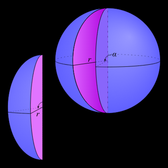
Figure 1. The Volume of a Spherical Wedge
As it turns out, the volume of the spherical wedge in figure 1 is to the volume of its sphere (actually ball) as the angle of the wedge is to 2π:
 ,
,
or, as the angle of the wedge in degrees is to 360 degrees.
So, in our case, the ratio 1/8 = 45/360.
This is not only interesting with respect to the wave equation, but also to the finding of Dave Lackey that the relative quark and lepton masses are related to definite angles of rotation. That these might be wedge angles seems highly likely to me.
The two figures below show the 2D rotation representation of the 3D oscillation graphically:
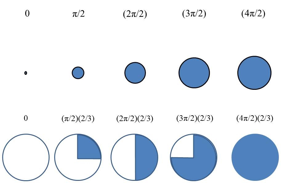
Figure 1. First 2π Rotation
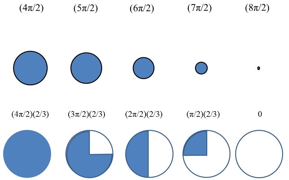
Figure 2. Second 2π Rotation
The reason this is so significant is that it provides a physical orgin of 4π quantum spin for the first time anywhere and also provides the basis for including the wave equation in our discrete system of theory.
Moving Forward
In the comments section, there’s been discussion about employing the wave equation in our research, expanding our outreach efforts and taking note of the work of Miles Mathis. In each case, I felt the resistance of initial inertia, but eventually began to experience some momentum building in my thoughts and feelings about these things.
Our immediate research goal here at the LRC is to arrive at the point where we can calculate the atomic spectra, using our RST-based theory (our RSt). The LST community’s ability to do this (well, in principle, anyway) and our inability to do it is embarassing. Nehru called it the “glaring lacuna” of Larson’s RSt (see here.)
While pursuing this goal, we’ve discovered many wonderful things, but none of them has enabled us to do the calculations yet. Perhaps, we may be finding ourselves agreeing with Nehru that the use of the wave equation may be inevitable after all, if we are going to reach our goal.
However, there are some intriguing conceptual developments that are closely related to the atomic spectra, which show the fundamental difference between the LST and the RST that has to be taken into account, if we are to use the wave equation in our calculations. The LST defines motion as a change in an object’s location, the distance between locations over the time it takes to travel that distance.
This idea of translational motion is extended to rotation, but the “distance” traveled is measured in terms of a time rate of change in the quantity of radians, or unit angles. We can count between the cardinal points on a circle, in terms of π:
t0…………t1…………t2………….t3…………..t4
0………(π/2)……….(2π/2)……….(3π/2)………(4π/2)
But when this convention was employed in quantum physics to describe quantum spin, it was found necessary to modify it to:
0……..(π/2)………(2π/2)………(3π/2)……..(4π/2)……..(5π/2)………(6π/2)………(7π/2)………(8π/2),
because one revolution of quantum spin requires twice as much rotation as one revolution of non-quantum spin, something not understood to this day in the LST community.
Since the LST concept of quantum spin, as incomprehensible as it is, was the key to the breakthrough of quantum physics in the LST community and its successful calculation of atomic spectra energy levels, it’s important to understand how it relates to the RST theory of atomic spectra energy levels, which has no concept of spinning electrons, whirling around a nucleus of protons and neutrons.
Moreover, in our LRC RSt, unlike in Larson’s RSt, and in Nehru’s modification of Larson’s RSt, there is no concept of rotation! Nehru sought to employ complex numbers to represent what he called “one-dimensional spin” in the time (inverse) region of the universe of motion, because time is 3D in this region and space is scalar. He also extended this approach to the use of quaternions to represent what he called “two-dimensional spin.” The 1D spin applies to what Nehru called the “Atomic Zone,” while the 2D spin applies to what he called the “Nuclear Zone.”
These time region studies see a 1D “electronic” potential between rotation in the complex plane and the 3D unit progression, and a 2D “nuclear” potential between the rotation of the 1D rotation itself in an orthogonal dimension and the universal progression. The former, is formulated in terms of 2D complex numbers, while the latter is formulated in terms of 4D quaternions. This follows pretty much the LST approach to calculating these potentials with Lie algebras, but replaces the LST concepts of the atom, such as electron clouds and nuclei, with RSt concepts of n-dimensional scalar rotations, forming the atoms, which oppose the universal expansion.
However, since the LRC RSt concept requires an initial 3D oscillation of the space (time) aspect of the progression, with compounds of the resulting entities forming the bosons and fermions of the universe of motion, we must find the corresponding “electronic” and “nuclear” potentials in these 3D entities, without recourse to n-dimensional “scalar rotations.”
Apparently, the way to proceed in our case is to extend the idea of Larson’s 1D scalar speed-displacements in a natural way, which we have tried our best to do, by first understanding the mathematics of scalar motion, which is manifestly different than that of vector motion. Three-dimensional scalar motion does not involve the changing location of an object, but the changing size of an oscillating volume.
This periodic change in volume occurs from postulated changes in the outward “direction” of the universal space/time expansion, at a given point in that expansion. We can express the unit 3D expansion in algebraic terms, by expanding Larson’s cube (LC) over time:
t0…………t1…………t2………….t3…………..t4
10…………23………..43………….63………….83
But the 3D ocillation, reversing at each unit, introduces a differential between it and the progression, which is determined by a given dimension of the oscillation. For its 1D component, for example, the 3D scalar expansion is:
11…………21………….41………….61………….81,
creating the unit speed-displacement in one dimension:
10…………out:21/(out:1x21)………..out:41/(in:2x21)………….out:61/(out:3x21)………….out:81/(in:4x21),
or a 1D unit speed-displacement: 1:2.
However, for the 2D component of the 3D scalar expansion, we get:
10…………22………..42………….62………….82,
creating a unit speed-displacement in two dimensions:
10…………22/(1x22)………..42/(2x22)………….62/(3x22)………….82/(4x22),
or a 2D unit speed-displacement:12:22.
For the 3D component of the scalar expansion, we get:
10…………23………..43………….63………….83,
creating a unit speed-displacement in three dimensions:
10…………23/(1x23)………..43/(2x23)………….63/(3x23)………….83/(4x23),
or a 3D unit speed-displacement:13:23.
This shows we’re in the game and what’s more, the discovery of Miles Mathis that π = 4, in kinematic equations, places the 3D potential squarely in our Wheel of Motion, as each group of elements follows a 4n2 , or a πn2 relation.
But we need to quantify the physical expansion/contraction using continuous magnitudes, since nature doesn’t expand by cubes. One way to do this is to divide the volume of the unit ball into 8 sub-unit balls that have a volume corresponding to the 8 1-unit cubes in the 23 stack of unit cubes of the LC.
The volume of the unit ball is just 4π/3, since r = 1. Thus, (4π/3)/8 is the sub-unit volume we need, and, as it turns out, the radius of this 1/8 volume is just the cube root of its ratio to the unit volume, or the cube root of 1/8, which is 1/2.
V1 = (4π/3), V2 = V1/8
V2 = (4π/3)r3
r3 = (V2/V1) = 1/8
r = (1/8)1/3 = .5
Now, if we map these sub-unit volumes (SV) to angles of rotation of the unit circle, we can construct a rotational analog of the volume oscillation. Our first four points of reference on the unit circle for the first four volumes are:
SV0…..SV1…..SV2…..SV3……SV4.
and our first four angles of rotation are:
0………(π/2)……….(2π/2)……….(3π/2)……….(4π/2),
Happily, 1/8th of the unit volume is equal to (π/2)/3, so our 3D scalar to 2D rotation map is:
0…..(π/2)(2/3)……(2π/2)(2/3)…..(3π/2)(2/3)…..(4π/2)(2/3)
which fills from 0 to unit volume in 1 unit of time, the expansion, and then the contraction deflates, from unit volume back to the starting point (0), taking another unit of time:
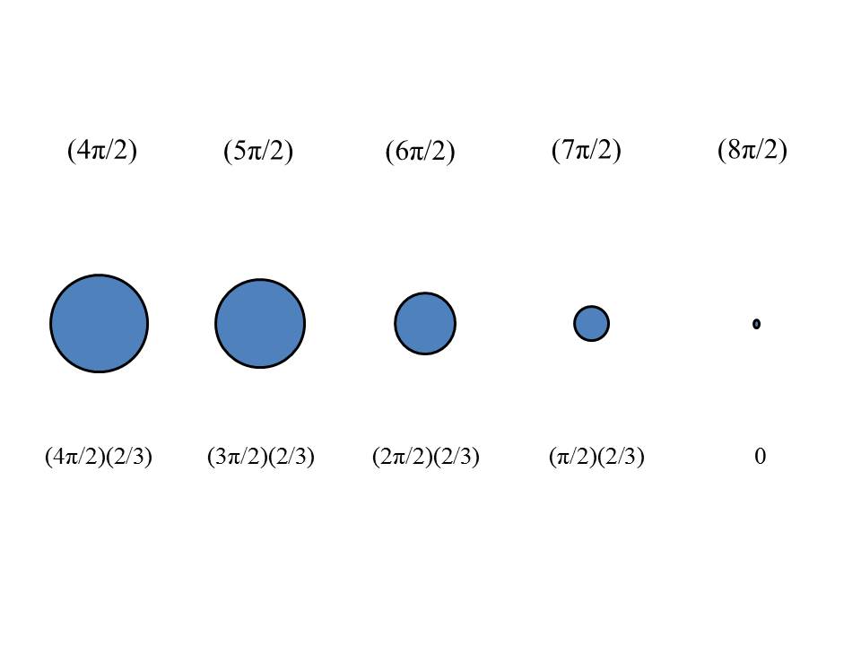
(4π/2)………(5π/2)……….(6π/2)……….(7π/2)……….(8π/2),
(4π/2)(2/3)…..(3π/2)(2/3)……(2π/2)(2/3)……..(π/2)(2/3)……….0
This is a significant achievement of the RST. Bruce Schaumm, on page 187 of his book, Deep Down Things, linked above, writes:
We don’t really have a clue about the physical origin of [quantum] spin. To describe spin as “intrinsic angular momentum” is like your best buddy describing how your car’s differential works by explaining that it “employs a mechanical linkage;” the only useful information contained in this statement is that its author probably knows next to nothing about how a differential actually works.
Well, it’s not all that hard to explain in the universe of motion:
The reason it seems that it takes two 2π revolutions to complete one cycle of quantum spin is that the “spin” is not actually 1D rotation, in 2D space, but the 3D oscillation of a volume in 3D space, as depicted below:
In the equivalent of one revolution of 2π, the 3D oscillation has fully expanded, which is one-half of its cycle. To return to the starting point at zero, requires a second unit of time, and the equivalent of a second 2π revolution. With this map of 3D oscillation to 2D rotation, we ought to be able to adapt the wave equation to move forward in the goal to calculate the atomic spectra.
UPDATE: As (π/2)/3 = .523598… = V1/8, two of these volumes, or V = (π/2)(2/3), are the equivalent of one π/2 rotation (90o.)
2nd Update: The above update is in error, since (π/2)/3 = .523598… radians = V1/8 = 30 degrees, not 45 degrees. Hence, the calculations shown are incorrect. The correct calculations are shown below:
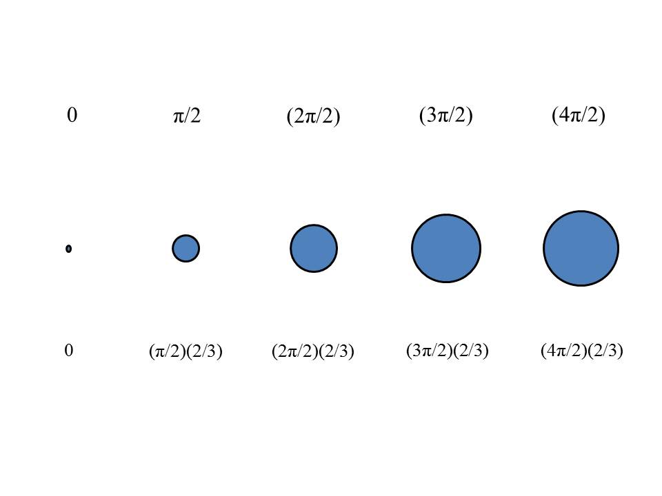
If we map these 8 sub-unit volumes (SV) to 4, 90, degree segments of 2π rotation of the unit circle, we can construct a rotational analog of the volume oscillation. Our first 4 points of 90 degree reference on the unit circle for the first 4 sub volumes are:
SV0…..SV1…..SV2…..SV3……SV4
and our first 4 segments of 90 degree equivalent rotation are:
0………(π/2)……….(2(π/2))……….(3(π/2))……….(4(π/2)),
Mapping the 1/4 volume to π/2 radian of rotation, the required delta in volume per 90 degrees of rotation, gives us .66667 volume units per 90 degrees of rotation:
V/x = π/2
x/V = 2/π
x = V(2/π)
x = 2.6666,
V/x = 4.18879/2.66667 = .66667 volume units, per 90 degrees of rotation.
Hence, the value of the 8 SVs in the original calculation does not correspond to the four, 90 degree rotations, as indicated in the graphic. In terms of radians, each of the 8 SVs is equivalent to 30 degrees of rotation, not 90.
Therefore, each delta in volume, corresponding to 90 degrees of rotation has nothing to do with the eight sub-volumes in the LC.
Instead,
0……..(π/2)………..(2(π/2))……….(3(π/2))……….(4(π/2)) =
0…..(.66667)…..(2(.66667))…..(3(.66667))…..(4(.66667)),
which fills the volume from 0 to unit volume in 1 unit of time, the expansion, and then the contraction deflates, from unit volume back to the starting point (0), taking one more unit of time, for a total of 360 degrees of equivalent rotation, per cycle, but taking two cycles, or 720 degrees of equivalent rotation, to return to the starting point (0):
(4(π/2))…………..(5(π/2))…………(6(π/2))…………(7(π/2))………(8(π/2)) =
(4(.66667))…..(3(.66667))……(2(.66667))……..(.66667)……………0
I’ll correct the graphic later.