The New Physics
The Scalar Mathematics of the Periodic Table (Continued)
In the previous post, we really never got into the scalar mathematics of the periodic table. That entry probably should have been entitled “the reciprocal mathematics related to the scalar mathematics of the periodic table!”
What we are trying to get at is the non-QM mathematics of the periodic table. Mathematics not based on the Shroedinger equation. Indeed, mathematics not based on complex numbers or the non-commutative numbers of QM.
Larson’s fundamental postulate excluded non-commutative mathematics, so he didn’t use complex numbers in his system of theory, but the theories of the legacy system of physical theory (LST) community are founded on non-commutative complex numbers. All of its research is based on the foundation of complex numbers, which employs the ad hoc invention of the square root of -1.
Of course, asserting that we should re-examine the use of imaginary numbers at this point in the game will relegate you to a permanent seat in the peanut gallery, if not a bed in a mental hospital, if you seriously pursue the idea.
Nevertheless, I am convinced that, unless we do just that, we will never be able to progress past the string theory impasse of today. Larson’s Reciprocal System of Physical Theory (RST) gives us the perfect opportunity and rationale to look at it seriously, as I have discussed in previous posts.
In our case, we started with Larson’s Cube, added the inner and outer spheres to it and were then able to construct a new scalar number line, a 3D number line, if you will, that necessarily contains the corresponding 2D and 1D numbers as well and conforms perfectly with the dimensional properties of the tetraktys and the inverse tetraktys.
Constructing magnitudes and algebras on this unique, multi-dimensional, scalar, number line should prove fruitful for the investigations of the RST, beginning with the periodic table and its associated atomic spectra.
Without this new number line, it’s difficult to understand the relations of the 2n2 and 4n2 integer patterns of the quantum numbers and their associated non-integer energy values, but with its additional properties, we might make some progress.
This is especially so given Le Cornec’s new and astonishing empirical discovery that the relative square roots of the energy values form a linear pattern that does not fit the QM atomic spectra pattern (see here). When we take the 4n2 mathematical pattern, we get four element slots in the first group of elements (n=1), 16 slots in the second group (n=2), 36 in the third (n=3), and 64 in the fourth (n=4), where each are subgrouped into two halves of the wheel, the two, 2n2, sub-patterns.
These sub-patterns follow our new scalar number line of 21/2, 81/2, 181/2, 321/2, and when we divide each of these by half its inverse, we get the 4n2 pattern of the number of elements in each of the successive circles of the Wheel of Motion: 4, 16, 36, 64.
This is encouraging, but the question is, “What is the physical meaning of ‘half the inverse?’” Why should each element’s numerical value equal half the inverse of the first four numbers of our new number line? We also would like to know how the four spectra, or energy, values, s, p, d and f fit into this new analysis.
More later.
The Scalar Mathematics of the Periodic Table
 Doug
|
Doug
|
 Post a Comment
|
Post a Comment
|
 1 Reference
|
1 Reference
|  Email
|
Email
|  Print
Print
In the previous post, we discussed the “first and second ordering” of the periodic table, as described by physicist Albert Tarantola. The first ordering fits a 4n2 relationship, when the first four elements, hydrogen through beryllium, are placed in the first period, and the total number of elements is extended from 118 elements to 120 elements. Charles Janet proposed this table in 1929.
However, besides adding two additional, unknown, elements to the total of the table, his approach slides the noble elements out of their keystone positions, as especially evident in the Wheel of Motion form of Larson’s table. This is really not a problem, but one hopes it’s not the case intuitively, because it destroys the aesthetics of the wheel.
What’s most interesting about Janet’s analysis is that it agrees with Larson’s in that it places four slots in the first period (4*12 = 4), not two, as in the QM table (2*12 = 2.) However, Larson doesn’t fill these 2 empty slots at the beginning with full-blown elements, as does Janet, but instead he fills them with the proton, and the massless neutron. Thus, helium and deuterium are both in the first period and the “keystone” elements in the Wheel of Motion are the noble gases, completing their respective periods at the 6 and 12 o’clock positions in the concentric circles of the wheel.
Janet – 2,2|8,8|18,18|32,32
Larson – 2,2|8,8|18,18|32,32
QM – 0,2|8,8|18,18|32.32
Meanwhile, Hervé Le Cornec has shown, in what C. K. Whitney calls “a stunning demonstration,” that the atomic ionization potentials exhibit a strikingly simple underlying pattern. The new pattern reveals that, while the elements are indeed grouped into the four 4n2 periods (or eight 2n2 sub-periods) exhibited by all these tables, the s, p, d, and f energy levels of spectroscopy repeat themselves in a different sequence than they do in the quantum mechanics theory. Le Cornec’s empirical pattern is:
s | s-p, s-p | d-s-p, d-s-p | f-d-s-p, (f-d-s-p),
while the theoretical pattern from QM, based on the four quantum numbers, n, l, m, s, and several rules of selection, is:
s | s-p, s-p | s-d-p, s-d-p | s-f-d-p, s-f-d-p.
Janet’s sequential pattern is the same as QM, but the energy levels are grouped differently, requiring the addition of two more elements at the end of the sequence:
s, s | p-s, p-s | d-p-s, d-p-s | f-d-p-s, f-d-p-s.
Tarantola refers to the latter two patterns as a “first ordering, and the Le Cornec pattern as a “second ordering,” of elements, as if the two orderings were not mutually exclusive, but Le Cornec believes that his work, based on the square roots of the ratios of atomic number Z, with the atomic number of hydrogen (1), shows QM to be defective. Interestingly enough, the Le Cornec sequence cannot be regrouped to fit the Janet table, as can the QM sequence.
The reason why is because the Le Cornec sequence places the “s” before the “p” energy level, in all periods, not just in the second, and both the “d” and the “f” levels in the third and fourth periods occur before the “s” and “p” levels, not between them, suggesting that the science of quantum mechanics is still not settled, and that the Schrodinger equation’s complexity hides an unknown, yet simple mathematical structure that organizes all atomic ionization potential (AIP) data.
Of course, this is exactly what we are looking for at the LRC, since, with our new, reciprocal, numbers, based on 1D, 2D and 3D pseudoscalars, and the recent discovery of how they fit so naturally into the tetraktys, giving us a non-pathological, multi-dimensional, algebra, we hope to demonstrate how this pattern of AIPs emerges from the natural sequence of these numbers; that is, we hope to be able to show that the periodicity of the periodic table, and the pattern of energy levels that forms it, are simply the result of nature counting from 1 to 4, using a ratio of pseudoscalars, not scalars.
However, the mathematical pattern of the periods is not the only thing we need to understand. While the right lines and circles inherent in the Euclidean geometry of Larson’s cube provides us with the multidimensional algebra with which to formulate the initial units, combinations of these units and the mathematical relations between them, we still need to quantify these units. We need to assign physical magnitudes to these mathematical units.
The magnitude of the RST’s universal motion, relative to its matter, depends upon the magnitude of the discrete space and time units that we select. Larson’s approach was to use the Rydberg frequency, R, and the speed of light, c, for this purpose. Since the constant speed of light plays such a central role in physical phenomena, it is reasonable to assume that the magnitude of the unit ratio, ds/dt = 1/1, is equal to c. This means that, if we can find the correct magnitude of either the space unit, or the time unit, we can easily calculate the magnitude of the reciprocal aspect.
Larson selected the Rydberg constant for this purpose, since it also seems to play a central role in the spectral phenomena of the hydrogen atom. The Rydberg frequency is 3.2899 x 10¹⁵ Hertz, so the reciprocal of this frequency is a time unit equal to 3.03961 x 10⁻¹⁶ seconds. The accepted value of the Rydberg constant has changed slightly since Larson’s day, so this figure differs slightly from his.
Since the units are vibrational, the actual unit of time, which Larson called the natural unit of time, that enters into the unit progression ratio, is half of this value (1/2 cycle), which he calculated as 1.520655 x 10⁻¹⁶ seconds, as found in his publications. Hence, the natural unit of space is then calculated as c divided by this quantity of time, or 4.558816 x 10⁻⁶ cm. So, the physical situation, at this point, is a constant increase of space/time, in three dimensions, the magnitude of which is 2.997930 x 1010 cm/sec, the speed of light, measured relative to matter (here, I use the figures in Larson’s publications, which, again, have been slightly modified since his day.)
While this seems to be a reasonable approach for deriving the magnitude of the discrete units, it’s never been directly substantiated, as far as I know. What’s more, at first blush, if the speed of light, s/t = 2.997930 x 1010 cm/sec, is the unit speed of the 3D expansion, as measured by the increase of its spatial radius, the RST’s inverse of this, t/s = 3.335635 x 10⁻¹¹ sec/cm, would be its unit inverse-speed, as measured by the increase of the radius of its temporal expansion.
Now, if we take Larson’s view of the radiation energy equation, E = hv, where the frequency term 1/t is cast as a velocity, with dimensions s/t, instead of 1/t, forcing the dimensions of Planck’s constant, h, to be t2/s2, as a consequence, then we have a velocity to work with, and the task to explain the meaning of the new dimensions.
One view we can take is that Larson’s modifications of the dimensions of frequency and Planck’s constant gives us a new understanding of the relationship of what we might call Einstein’s constant, s2/t2, and its inverse, what we will now call Larson’s constant, t2/s2.
Since the dimensions of mass, t3/s3, are related to energy, t/s, by Einstein’s constant, then it’s a logical conclusion that the dimensions of inverse mass, s3/t3, are related to velocity, s/t, by Larson’s constant.
This is tantamount to asserting that Einstein’s mass-energy equation, E = mc2, is just the reciprocal of an inverse-mass-energy equation, 1/E = (1/m)(1/c)2, even though Larson never really wrote this equation down, as far as I know. In other words, 1D energy is equal to 3D energy (mass) times Einstein’s constant, while 1D “velocity” (radiation) is equal to 3D velocity (inverse mass) times Larson’s constant.
However, the fact that, in the development of the theory, we have to convert the 1D velocity, s/t, into a frequency, 1/t, via “directional” reversals, in order to transform it into a quantum unit, while we don’t have to convert the 1D energy, t/s, into a frequency, 1/s, in order to transform it into a quantum unit, causes us to wonder why. Could it be that the dimensions, t/s, can be expressed as a spatial frequency, 1/s, with a temporal wavelength, analogous to the spatial wavelength of the 1/t temporal frequency?
If the answer to this question is yes, as the RST strongly implies, then the spatial-radiation energy equation 1/E = (1/h)(1/v) —> s/t = s2/t * 1/s, the inverse of the temporal-radiation energy equation, E = hv —> t/s = t2/s * 1/t, would also hold.
But even if the mathematical operations make sense, that fact doesn’t necessarily mean that the physical operation makes sense. Even if we can make sense of a conversion from frequency to velocity, and vice-versa, what is inverse energy? We know dimensionally, this term is velocity, but the LST community’s question would be, “Velocity of what?”
For the RST community, however, a quantity of s/t motion is just as viable as a quantity of t/s inverse-motion. When Einstein’s equation was discovered, it didn’t take long to find a way to transform mass into energy and check it, but how do we find a way to check the inverse equation? I have some ideas.
Square Roots & 1st & 2nd Orderings of the Periodic Table
In 1929, Charles Janet published his paper, “Deliberations on the Structure of the Nuclear Atom,” in which he proposed an interesting alternative to today’s Periodic Table of Elements. Although it has been almost completely ignored, his table was loosely based on the same 2n2 periodic relationship used in quantum mechanics, but, as shown in figure 1 below, with an interesting twist. The first period contains four elements!
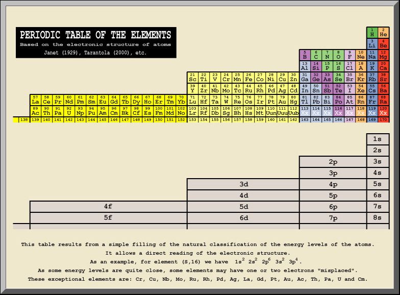
Figure 1. The Periodic Table of Charles Janet Published in 1929.
This table, appearing on Albert Tarantola’s website, is based on Janet’s work, which Tarantola refers to as the “first ordering” of the elements. It follows the accepted electron configuration sequence in ascending atomic order, so even though the two columns of akali metals and akaline earth metals are moved over to the right under hydrogen and helium, the accepted order of electron shell filling is maintained, as shown in table 1 below.
|
|
|
|
1s |
|
|
|
|
2s |
|
|
|
2p |
3s |
|
|
|
3p |
4s |
|
|
3d |
4p |
5s |
|
|
4d |
5p |
6s |
|
4f |
5d |
6p |
7s |
|
5f |
6d |
7p |
8s |
Table 1. Z-Ordered Electron Configuration of Janet Table (Read left to right, top to bottom)
This is interesting in the context of the LRC’s RST-based research, because the periods of Larson’s periodic table (here) are based on his 4n2 relationship, which requires four elements in the first period. Of course, it’s always been assumed that the three missing elements in the first period were incomplete elements such as the proton, neutron and electron (or neutrino, or massless neutron, etc.)
However, the placing of helium, lithium and beryllium into the first period is very interesting, although it “dethrones the noble gases from their key positions in the table, which is especially disappointing in view of the LRC’s Wheel of Motion form of the table.
Interestingly, as Tarantola and others have pointed out, another form of the table can be constructed from a ratio of square roots of atomic ionization potentials, as first shown by Le Cornec in 2002, using actual ionization data from the existing literature. Although Tarantola dismisses the significance of Le Cornec’s work, because he offers no theory to explain it, he does acknowledge that it shows a reversal in the order of the “s” and “p” energy levels, which, unlike Le Cornec, who asserts that this indicates a major failure of quantum mechanics, he simply attributes to the fact that the atom is a “complex object.” Tarantola calls this table the “second ordering” and leaves it at that.
For us, though, the fact that the ionization pattern shows a different order, inconsistent with the standard atomic model, is extremely interesting. One of the reasons why appears in the mapping of the s, p, d and f energy levels to the tetraktys. If we place these sets of 2 energy levels into the tetraktys, with subscripts indicating each, we get table 2 below.
|
|
|
|
2s |
|
|
|
|
|
|
2s |
|
2p |
|
|
|
|
2s |
|
2p |
|
2d |
|
|
2s |
|
2p |
|
2d |
|
2f |
Table 2. Duality of Electron Configurations Mapped to the Duality of the Tetraktys
As will be readily noticed, the energy levels map perfectly to the tetraktys, in some respects. There is one of the four dual “s” sets at the top, with the remaining three “s” sets positioned in the same repeating fashion, at the beginning of each row, as the 20 values in the tetraktys. The total number of sets is consistent as well, with four dual “s” sets, three dual “p” sets, two dual “d” sets and 1 dual “f” set, each set having two, six, ten and fourteen members, respectively (the difference between the successive 2n2 periods), arranged into four groups, corresponding to the four 4n2 periods of Larson’s table and the Wheel of Motion.
In fact, the only missing characteristic seems to be the accepted electron configuration order. However, Le Conec’s ionization’s order doesn’t comply either. As shown in figure 2 below, Tarantola’s table of second ordering takes lithium and beryllium out of the first period and puts them back into the second period, as indicated by Le Cornec’s ionization results.
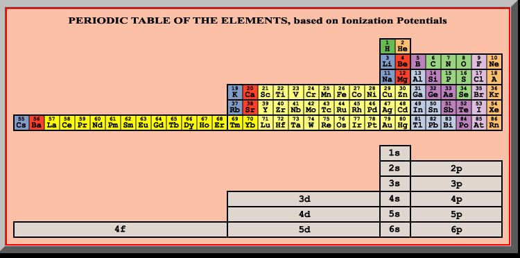
Figure 2. Tarantola’s Modification of the Periodic Table (Second Ordering) Given Le Cornec’s Results
But, if we take the fact that Janet’s table, based on a 2n2 period, concurs with Larson’s table, based on a 4n2 period, and the fact that Le Cornec’s results contradict quantum theory, based on a ratio of square roots, we have to take notice, because, as it turns out, the oscillating pseudoscalars (SUDRs & TUDRs) of the S|T units, contain both the 2n2 and the 4n2 terms, as the two factors in a series of ratios of square root products that fit the four periods of the table!
Again, the only thing missing is the order of the energy levels. If we map the four periods of the square root equations to the tetraktys, we get a perfect match, as shown in table 3 below.
|
|
|
|
2x4 |
|
|
|
|
|
|
2x4 |
|
8x16 |
|
|
|
|
2x4 |
|
8x16 |
|
18x36 |
|
|
2x4 |
|
8x16 |
|
18x36 |
|
32x64 |
Table 3. Duality of S|T 2n2 x 4n2 Periodicity Mapped to Tetraktys
Though, at first, this seems counter intuitive, it works because the equations of the table are based on the equation of inverse geometry (r’2 = r * r’’), where the inverse of a given circle’s, or sphere’s, radius, works out to be twice, or half, its radius. Students of the RST will recognize the significance of this immediately, since 1/2 and 2/1 are the basic units of speed-displacement in the system.
Details to follow soon.
The "Glaring Lacuna"
One of the most important and immediate objectives of our research here at the LRC is to address the “glaring lacuna” in Larson’s work, the inability to calculate the atomic spectra. Larson tried to work it out, but temporarily gave it up, when it appeared so complex and obtuse a subject that it became apparent that it would drain his resources and slow his progress in developing his RST-based theory, what we call his Reciprocal System theory (RSt).
It was Nehru who gave it the label with which we still refer to it today. While noting this great contrast with the success of the LST’s wave mechanics in explaining the “vast wealth of spectroscopic data,” he goes on to elaborate on the much heralded success of the LST theory:
The several quantum numbers, n, l, m, etc. come out in a natural way in the theory. Even the “selection rules” that govern the transitions from one energy state to another could be derived. The fine and the hyperfine structures of the spectra, the breadth and intensity of the lines, the effects of electric and magnetic forces on the spectra could all be derived with great accuracy. In addition, it predicts many non-classical phenomena, such as the tunneling through potential barriers or the phenomena connected with the phase, which found experimental verification.
Of course, all of this began with Heisenberg’s great discovery of the non-commutative multiplication in the first mathematical structure of quantum mechanics. As Bohr wrote Rutherford:
Heisenberg is a young German of gifts and achievement. In fact, because of his last work, prospects have at one stroke been realized, which, although only vaguely grasped, have for a long time been the center of our wishes. We now see the possibility of developing a quantitative theory of atomic structure.
In developing an RST-based theory, however, the second postulate limits us to an algebra of magnitudes that is ordered (absolute), commutative and associative (meaning its geometry is Euclidean). Nehru’s approach, an attempt to clarify the physical concepts of quantum mechanics, while keeping the mathematics, is therefore problematic, unless we drop the second fundamental postulate of the RST.
Fortunately, as described in the previous post, the new mathematics developed at the LRC, based on reciprocal numbers as analogs of the scalar/pseudoscalar ratios, maintains these essential algebraic properties. Using this algebra, we have been able to build a simple toy model of the motions and combinations of motions that is consistent with the second postulate and that contains the bosons and fermions (both quarks and leptons) of the standard model of particle physics and the baryons of the periodic table based on Larson’s 4n2 concept, as opposed to the 2n2 concept of quantum mechanics.
The challenge, however, has, again, been to identify the quantitative relations between these bosons, quarks and leptons, as observed in the experimental energy levels of the baryons. In short, we need the RST breakthrough that corresponds to Heisenberg’s quantum mechanical breakthrough.
Well, I’m happy to announce today that the needed breakthrough has arrived; at least it has as far as the toy model is concerned. Recall that our RST-based model, unlike the LST model and Nehru’s model, is not based on rotation, but rather the vibrations of the pseudoscalars, which we call S|T units, the SUDRs and TUDRs, which are inverse pseudoscalar/scalar oscillations. Figure 1 shows how these combine to form the entities of the standard model.
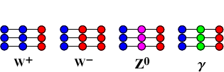
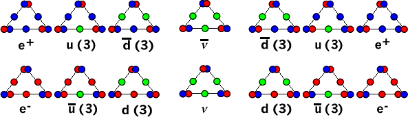
Figure 1. Scalar Motion Combinations
The middle colors, green, red and blue are used to indicate the relative balance of red SUDRs and blue TUDRs in a given combination. A green circle in the middle of a combo indicates an even number of each. A red color indicates more SUDRs than TUDRs, while a blue color indicates the reverse. We assume an initial value of one SUDR and one TUDR in the green balanced combo, and an excess of one kind of unit in the unbalanced combos.
This works out perfectly in terms of combining protons, neutrons and electrons, but the question has been how to fit the photons into these combos. In the quantum mechanical model, the electron is regarded as orbiting the nucleus (Bohr’s model), even though this was modified (the cloud model) to fit Heisenberg’s mathematical structure, wherein no definite orbital path could be identified.
In the S|T model, the electron doesn’t rotate around the nucleus, but becomes an integral part of the atomic structure, as shown in figure 2 below:
Electron

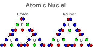
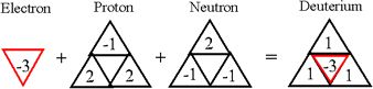
Figure 2. Combining Quarks and Leptons into Baryons
Even though the standard model is empirical, the mathematical relations of its entities are described by Heisenberg’s fundamental mathematical structure developed in two theories: The first theory is quantum electro dynamics (QED), and the second theory is quantum chromo dynamics (QCD). Both of these theories are based on rotations and suffer from the algebraic pathology of higher dimensional numbers, as explained in previous posts. The underlying mathematical structure is described as based upon the principles of symmetry in U(1)xSU(2)xSU(3) groups, but these groups are formed from numbers derived from rotations.
In our theory, there are no rotations, so the challenge has been how to show the different energy levels of the atomic spectra in the new model, which has no orbits or electron shells. The breakthrough has come by realizing that the combinations of motions in the S|T combos, while numerically balanced and accurate in the baryons and their combos are nevertheless what we might call internally polarized. This was understood by simply tabulating the SUDR|TUDR counts at the nodes of the combos. For instance, tabulating the S|T nodes in the combination of a proton, neutron and electron, as shown in figure 3a below, results in a polarized triangle, representing the deuterium atom, as shown in figure 3b.
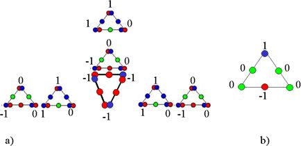
Figure 3. The Polarization of Non-Ionized Deuterium
This is a remarkable and fortuitous result, since it permits the binding of a boson to the atom, as shown in figure 4 below, without changing anything, but the energy of the combo:
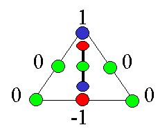
Figure 4. Combining Photons with Baryons
On this basis, we may now begin to develop a quantitative relation between photons and atoms in our model – the atomic spectra! Indeed, we might say that, perhaps, the prospects at one stroke have been realized, which have, for a long time, been the center of our wishes!
The Tetraktys and Oscillating Pseudoscalars
The importance of the tetraktys in mathematics and physics is well known, as the Clifford algebras are intimately associated with the study of geometry and physical theory. Here at the LRC, we know that this is due to the fact that the union of mathematics and physics requires understanding that there are three properties of numbers and motion: magnitude, dimension and “direction,” where each non-zero dimension has magnitude in two “directions,” which we can think of as up and down, left and right, forward and backward.
The fact that rational numbers and scalar motion have inverses (two “directions”) means that the tetraktys should also have its inverse, and, in fact, it does. We can show this by writing the numbers of the tetraktys as ratios:
20/20 = 1/1
20/20 21/20 = 1/1, 2/1
20/20 21/20 22/20 = 1/1, 2/1, 4/1
20/20 21/20 22/20 23/20 = 1/1, 2/1, 4/1, 8/1
then its inverse is obviously,
20/20 = 1/1
20/20 20/21 = 1/1, 1/2
20/20 20/21 20/22 = 1/1, 1/2, 1/4
20/20 20/21 20/22 20/23 = 1/1, 1/2, 1/4, 1/8
This may not be of interest to the LST community, because they don’t recognize scalar motion, let alone multi-dimensional scalar motion, and even if they did no doubt they would be stopped cold by the notion of super-luminal speeds.
But in the RST community, aware of the cosmic sector and its inverse speeds, the inverse tetraktys is of great interest, since it is a generalization of the multi-dimensional numbers, and their algebras, of the cosmic sector, just as the tetraktys is the generalization of those things in the material sector.
To truly understand the theoretical universe of the RST, both the tetraktys and the inverse tetraktys are necessary. Of course, this means that we need multi-dimensional numbers and units of motion that are scalar, or pseudoscalar, but, unfortunately, these don’t exist in the LST community’s system of mathematics. They have devised an imaginary number (the so-called square root of -1) to raise the dimension of scalar numbers, because they needed to stick with the 1D motion of objects, not realizing that motion without objects is also possible.
However, as we know, this has sickened their multi-dimensional algebras, forcing them to cope with trying to understand physics with nothing but scalars and vectors, or the 0D numbers of scalars and the 1D numbers of complex numbers. Because of this, most physicists and engineers would think we’ve gone batty if we start referring to multi-dimensional scalars - to them, it’s a contradiction in terms.
Nevertheless, that’s really what pseudoscalars are. So now we want to go back and replace the imaginary square root of -1, upon which the superstructure of modern mathematics has been built, with the square root of 2, which is not an imaginary number, but a very real one (no pun intended here - lol).
The way I hope we can do that is, first, by recognizing that the 3D pseudoscalar has all the properties we need to coax matter out of scalar motion: Like the 3D gravitational property of matter, with its two “directions,” in and out, the 3D pseudoscalar has 3D volume with two “directions,” expansion and contraction. Likewise, the 2D magnetic property of matter, with its two “directions,” north and south, is analogous to the 3D pseudoscalar’s 2D surface, having an inner and outer side, which cannot be separated. Finally, the 1D electrical property of matter, with its two “directions,” positive and negative, is reflected in the 3D pseudoscalar’s 1D circumference, which also has two “directions,” clockwise and counter-clockwise.
Add to this the fact that the inverse pseudoscalar is already studied in the field of inversive geometry, and we have at least two good reasons to suspect that this line of investigation is worth pursuing.
As explained recently in the New Math blog (See here), the square root of 2 turns out to be quite useful for defining numbers, in terms of the geometry of the three spheres, which correspond to -1, 0, +1, when -1 is understood to be 1, 0 is understood to be the square root of 2, and +1 is understood to be 2, the inverse of 1, and we replace these integers with the rational numbers, 1/2, 1/1, 2/1, using Larson’s concept of speed-displacement.
This may sound crazy at first, but it’s only necessary to understand that 0 doesn’t really have to be understood in the way it’s normally portrayed on the real number line, or in Cartesian coordinates. That is to say, the way we understand it in our LRC research is not like this:
-n …, -3, -2, -1, - 1/2, -1/3, … -1/n, 0, 1/n…1/4, 1/3, 1/2, 1, 2, 3, … n
where the unit distance is seen as infinitely divisible, but rather as,
1/n, …1/4, 1/3, 1/2, 1/1, 2/1, 3/1, 4/1, …n/1
where each unit is not infinitely divisible, but is discrete and has its discrete inverse unit, as in group theory. In this way, 0 does not have a place on the number line per se. Instead, it is implied by 1/1 = 0, when the binary operation of the group is changed from multiplication to addition, and the meaning of the “/” symbol becomes a “displacement” operation between the numerator and denominator, not an inverse multiplication operator.
With this much understood, we want to map the set of pseudoscalars, corresponding to the first two units of the expansion (t1-t0 = 1 and t2-t0 = 2), to the tetraktys and the inverse tetraktys, in the same way we map the rational numbers to it, using the intermediate pseudoscalar, with the unit ratio of the square root of 2, as the 0D tetraktys value, the ratio of the 1D circumferences as its 1D value, the ratio of the 2D surfaces as its 2D value, and the ratio of the 3D volumes as its 3D value.
We can use circles with differing patterns to indicate which aspect of the spheres is being symbolized, a pattern of dots for the 0D pseudoscalar, a pattern of lines for the 1D one, a pattern of squares for the 2D one, and a solid fill for the 3D one, as shown below:
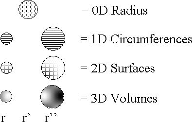
Figure 1. Symbolic Notation for Radii, Circumferences, Surfaces and Volumes of Pseudoscalar Spheres with Radii r =1, r’ = (2)1/2, r’’ = 2.
First, we construct the pseudoscalar tetraktys, then the inverse pseudoscalar tetraktys:
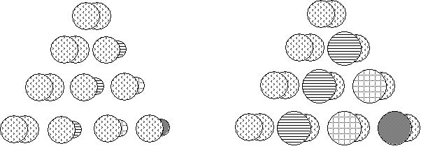
Figure 2. The Tetraktys and Inverse Tetraktys of Pseudoscalar Sphere Ratios
As it turns out, each of these pseudoscalar ratios is a power of the square root of 2. The unit ratio, which is just the ratio of the radius r’ to itself, or the square root of 2, divided by itself, is equal to 1. Letting R equal this unit ratio, we can write it as R0 = (21/2)0 = 1, because any number raised to the zero power is equal to 1. The ratio of the 1D circumferences of r’ and r, 2πr’/2πr, is equal to the square root of 2, or (21/2)1, which we can write as R1. The ratio of the 2D surfaces, 4πr’2/4πr2, is equal to 2, or (21/2)2, which we can write as R2. Finally, the ratio of the volumes, (4/3)πr’3/(4/3)πr3, is equal to 2*21/2, which we can write as R3, since 2 * 21/2 = (21/2)3.
Substituting these values of R for the graphics shown in figure 2, we can rewrite the pseudoscalar tetraktys, and its inverse, symbolically, as shown in figure 3 below:
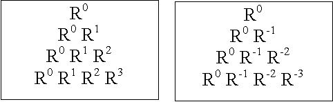
Figure 3. The Symbolic Pseudoscalar Tetraktys and Its Symbolic Inverse
This is a remarkable result, because it appears to constitute the basis for a multi-dimensional number system with no algebraic pathology, since each associated pseudoscalar algebra would presumably be as completely ordered, commutative and associative, as the well known scalar algebra.
Clearly, the R0 numbers are ordered, since the square root of 2 is a real number. The R1 numbers are ordered, because we can’t have an R1 number smaller than 1. The R2 numbers and the R3 numbers are also ordered for the same reason, because no areas and volumes smaller than the unit areas and volumes exist in the system, by definition.
Indeed, I think the proof that all these numbers are ordered, commutative and associative is trivial, so I won’t bother to show it here.
Of course, I could be wrong – and very embarrassed – again!