The Larson Research Center

Note: This article was inadvertently published on March 3rd, before it was completed. The completed article was published two days later, on March 5th.  

In the previous post, we discussed the effect the Chart of Motions (CM) has on the concept of the so-called incommensurable, or irrational, numbers.  In short, when it’s realized that the concepts of numbers and magnitudes are naturally unified, we see that there is no need for the ad hoc inventions of real, imaginary, and compactified numbers.  However, this is a startling conclusion, given that the whole of modern science and technology is built on the use of these ad hoc concepts, and, as they say, extraordinary claims demand extraordinary proof.

Nevertheless, while it’s true, at the moment, that we don’t have the necessary proof, but are only conjecturing that this is the case, having a rational basis for making such a conjecture (no pun intended) is still impressive. The foundation of the claim rests on Larson’s discovery that the nature of space is not the distance, area, or volume defined by a set of points, satisfying the postulates of geometry, but rather the reciprocal of time, in the equation of motion.  This discovery changes everything, and it changes it profoundly.

We know that time marches on incessantly, independently, regardless of observation or agency.  Now Larson’s work shows us that, if the march of time is endless, then there must be a, reciprocal, march of space as well.  In other words, the observation of the universal, eternal, increase of time, tells us that there must be a universal, eternal, increase of space as well, by definition.  In short, there is a universal, eternal, motion in nature.  In fact, we can measure both the time aspect and the space aspect of this motion, by observing distant galaxies with powerful telescopes, as Hubble was the first to discover.

There are many consequences of recognizing this new, universal, motion, but one of the most important, and relevant to understanding numbers, is that what we call “distance” between points is not space that exists independently and that has any kind of properties.  The proof of this is that space cannot be measured independently of time, and time cannot be measured independently of space.  To measure the distance between points, either in terms of space, or in terms of time, requires motion, or both space and time, reciprocally related.  In other words, to measure, or calculate, the distance between physical points in a coordinate system, the motion that separated the points, or will separate the points, must be measured. 

The magnitude of the motion measured is not necessarily important, unless it is used as the basis for calculation.  For instance, if measuring the distance by eye (perspective) the speed of the light traveling over the distance is not important, or, if measuring by a standard rod or tape, the speed of the act of placing the device between physical points is not important, but motion of some magnitude must take place between the points, in order to measure (estimate) the distance. On the other hand, If time is used to measure the distance, as when timing the motion between the points, then the speed of the motion must be known in order to calculate the distance, as when lasers, radar, or sonar are used to measure distance.

Without exception, however, distance cannot be measured independently.  It is the space aspect of motion that must be determined, in order to measure the distance between points.  What this implies, as explained in the previous post below, is that there is not a one-to-one correspondence between numbers and the infinite points of a continuum, as assumed by most, and as regarded as “consummated” by the work of Cantor-Dedekind.

The fundamental postulate of the Cantor-Dedekind complete ordered field, which constitutes the so-called real numbers, is that the geometric linear continuum corresponds to the arithmetized real continuum,  where there is an irrational number between every pair of rational numbers, and a rational number between every pair of irrational numbers, leaving no gaps, if you will.  However, now we see that if there is no continuum of points in space, as assumed, but only motion that can be measured, then the need for a continuous set of numbers with no gaps makes no sense.  What needs to be “complete” is the set of ordered motion magnitudes, not a set of ordered space magnitudes.

Wikipedia describes the “Dedekind-cut” basis for real numbers as follows:

The Dedekind cut resolves the contradiction between the continuous nature of the number line continuum and the discrete nature of the numbers themselves. Wherever a cut occurs and it is not on a real rational number, an irrational number…is created by the mathematician. Through the use of this device, there is considered to be a real number, either rational or irrational, at every point on the number line continuum, with no discontinuity.

Of course, the reason the legacy system of mathematics (LSM) mathematicians feel the need to create irrational numbers is their assumption that a “number line continuum, with no discontinuity,” is required, because they assume that the physical magnitudes between points is space and that space is continuous, and therefore they reason that the discrete concept of number must be changed to correspond to the continuous concept of space magnitude.  However, the assumption of the RST is that the distance between points is the space aspect of motion and that the fundamental form of these magnitudes is both discrete and continuous, therefore it follows that, in a universe of nothing but motion, there is no need of ad hoc irrational numbers.

Another way to look at what is happening is to consider a Cauchy sequence as the basis for creating irrational numbers.  A Cauchy sequence is a sequence of rational numbers whose elements become closer as the sequence progresses.  In other words, the sequence should converge on the “real number line continuum,” meaning that a metric “space” in which all Cauchy sequences converge to the limit, a necessary concept of calculus, can be called complete. However, the only way to make a sequence of rational numbers converge completely (“to the limit,” as they say), thus corresponding to the continuity of a metric “space,” or measurable distance, is to include the invention of irrational numbers along with rational numbers in the set of real numbers.

By defining a Euclidean metric “space,” or distance, in terms of a function, called a “norm,” Pythagoras’ theorem can be used, as the defining function, in which the hypotenuse of a right triangle defines the “space” measure, or metric. Thus,

1) a² + b² = c² 

when a and b are real numbers, constitutes both the rational and irrational, or “real,” set of numbers.  In other words, any value of c can be expressed as a function of a and b, but only if a and b are allowed to be both rational and irrational, or real, numbers, and not if a and b are limited to rational numbers.

With the light of the new RSM, however, which incorporates the reciprocity concepts of the RST, the apparent incommensurability, inherent in the multi-dimensional numbers of the Pythagorean theorem, is completely misleading. What’s not commensurable is the idea of a continuum of motion and a continuum of space, not continuous space magnitudes and discrete numbers. If there is no independent space, then there is no continuum of space, and, therefore, there does not need to be a continuum of numbers that is in a one-to-one correspondence with the points on a line.  What needs to be logically complete is the discrete set of possible numbers that corresponds to the discrete set of possible physical magnitudes of motion, not the continuous set of possible numbers that corresponds to a continuous set of possible physical points of space.

Nevertheless, without the concepts of motion clarified by the CM, the fact that the change of position motion (M₂ motion) can take any one of an infinitely continuous range of values, not just a set of discrete values, argues to the contrary.  It is only when we recognize the differences between the three types of motion, M₂, M₃, and M₄, and how they relate to one another, that we can comprehend how discrete values of magnitudes of M₄ motion can make continuous values of M₂ motion possible.

It’s not difficult to understand this in a universe of nothing but motion, because, in such a universe, points in metric space don’t exist apriori.  To define metric space, one must define points first, and the only way to define points, in a universe of motion, is through discrete magnitudes of motion.  In the CM, we see that discrete points are defined by discrete magnitudes of M₄ motion.  Therefore, it follows that M₄ motion must precede M₂ motion.  Once two, or more, such discrete points exist, the separation of their locations is a measure of the past motion that separated them, which can be M₄ or M₂ motion.

Consequently, we may regard M₄ magnitudes, as more fundamental than M₂ magnitudes of motion, and it then follows that it is these discrete magnitudes of M₄ motion that discrete numbers should correspond to, not the continuous magnitudes of M₂ motion.  Fortunately, this appears to be the case.

We find that the insight of the universal progression, from which we assume the entire structure of the physical universe is derived, gives us a clear understanding that, contrary to LSM concepts, the natural numbers do indeed have the three properties of magnitude:

1. Quantity
2. Duality
3. Dimension

In order to understand this, the use of the RSM’s operational interpretation (OI) of number is required, wherein a “norm” of magnitude is defined by a function,

2) m|n = i

where m and n are natural numbers and i is the difference between m and n, called a displacement.  When m > n, i is positive. When m < n, i is negative.  When m = n, i is zero.  The operator, ‘|’, is used in a similar manner as the division operator, ‘/’, but does not signify a quotient, but only a reciprocal relation between m and n, the value of i.  Thus,

3) |m|n| = |n|m|

or the absolute value, the displacement of  -i, is equal to the absolute value, or displacement, of i.  Given OI numbers, the equation

4) m|n = 1|1 = 0 

is regarded as a statement of equivalence, such that m has the same, but inverse, value of n, as do equal weights on a pan balance, zero indicating the balance between equal magnitudes, similar to the financial concepts of debits and credits, where a series of transactions results in debts and assets that are calculated on a balance sheet, to determine the net worth of an individual, at a given point in time.

However, while OI numbers are not dynamic themselves, they can nevertheless represent relative rates of change, and, thus, changes in relative rates of change.  But this brings up an interesting aspect of OI numbers.  Whereas, in the traditional quantitative interpretation (QI) of number, used in the LSM, there is no difference in the numbers

5) 1/1 = 2/2 = 3/3 = n/n,

there is a difference in the OI case,

6) 1|1 < 2|2 < 3|3 < n|n,

just as there is a difference between the debts and assets of a millionaire and a pauper, even though the net worth of each can be the same, namely zero, whenever their respective debts and assets are equal. Consequently, this fact implies that the OI numbers are ordered, in increasing order, as shown in the sequence of equation 6), unlike the QI numbers in the sequence of equation 5). Furthermore, we can see that the numbers of equation 6) are ordered by size, because each successive number in the sequence contains one more possibility of distribution than its predecessor, just as n units of weight on a pan balance do.

In a pan balance, there is no freedom of choice for weighing 1|1, but there is one degree of freedom for weighing 2|2, two for 3|3, and so on; that is, in the case of 2|2, the number can be balanced, or unbalanced by one unit, in either direction; for 3|3, the number can be balanced, or unbalanced by two units, in either direction.  This can be expressed as an increasing number of numerical combinations, using OI numbers, as,

(1|1); (1|2, 2|2, 2/1); (1|3, 2|3, 3|3, 3|2, 3|1)… 

That the number of possibilities, as n|n goes to infinity is complete is obvious. There are no other possibilities, yet these infinite possibilities are contained in unit values formed by n|n = 1, and, therefore, they can be regarded as increasing divisions of unity, just as much as the two terms of equation 1) are regarded, in the LSM, as the function defining the Euclidean norm of a space metric.  However, while the LSM mathematicians must create irrational numbers, in order for the numbers a and b to converge on all values of c, nothing has to be created in the RSM.

To see this more clearly, consider the LSM and RSM numbers lines depicted below:

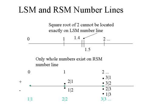
Figure 1. Two Number Lines

Again, the postulate of the real number system is that the geometric linear continuum corresponds to the arithmetized real continuum,  where there is an unidentifiable irrational number between every pair of rational numbers, and a rational number between every pair of unidentifiable irrational numbers, leaving no gaps.  In other words, the rational number line is incomplete.  To complete it, the idea of unidentifiable irrational numbers was defined, or invented, and, when added to the rational numbers, the irrational numbers complete the incomplete rational number line, which is then called the “real” number line.

However, as shown in figure 1 above, in the RSM, there exists another complete set of numbers that has nothing to do with the geometric linear continuum.  The OI numbers of the RSM form an infinite set of ordered numbers, each equal to 1.  In spite of this seeming contradiction, the elements of this ordered set actually constitute ordered subsets of denser and denser subdivisions of one, as can be clearly seen in the “meter” analogy of figure 2 below:

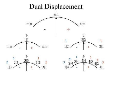
Figure 2. The Meter Analogy of OI Numbers 

In the “meter” at the top of figure 2, clearly there can be no displacement, because, 1 is not sub dividable, but 2 can be subdivided as shown, 3 even more so than 2, 4 more so than 3,  and so on, with each successive number in the set being more sub dividable than its predecessor.  Each number in the order is more sub dividable, thus larger, than the previous number.

That the ordered set is complete is easily seen in that there are no other possibilities between the successive numbers, unlike the infinite points on a geometric linear continuum, where there always must be a midpoint between any two points.  Thus, we see that the invention of the “real” number system is a misguided attempt to force the discrete number system into a one-to-one correspondence with the points of the geometric linear continuum, when actually they form a different sort of continuum, a continuum of operationally interpreted ratios, if you will.

The next step is to show that this set of OI numbers is not only ordered and complete, but also constitutes a field.  However, we’ll have to address that subject later. 

In discussing the ancient Greek strategy of using the discrete counting numbers to represent continuous magnitudes of line segments, David Hestenes writes:

With admirable consistency, Euclid carefully distinguished between the two concepts. This is borne out by the fact that he proves many theorems twice, once for numbers and once for magnitudes. (See his New Foundations for Classical Mechanics)

The reason for making this distinction between the discrete numbers and the continuous magnitudes of line segments, and keeping them separate in calculations and proofs, is easy to understand, as soon as it’s recognized that measurements involve magnitudes for which there are no counting numbers. The magnitude of the diagonal of the unit square is the simplest example. Hestenes points out that the “Hindus and the Arabs resolved this difficulty directly, by generalizing their notion of number.” However, “Euclid,” he writes, “sidestepped it cleverly by re-expressing problems in arithmetic and algebra, as problems in geometry. Then, he solved for line segments instead of for numbers.”

Euclid’s “sidestepping” approach worked because he labeled products with geometric magnitudes, so that he could represent the product x², as a square with sides of magnitude x, the product xy, as the “rectangle” xy, and the product x³, as a cube with sides of magnitude x. However, Hestenes observes:

But there are no corresponding representations of x⁴ and higher powers of x in Greek geometry, so the Greek correspondence between algebra and geometry broke down. This “breakdown” impeded mathematical progress from antiquity until the seventeenth century, and its import is seldom recognized today.

However, while Hestenes cites this “geometric” approach of the Greeks as a major factor in the “long period of scientific stagnation” that occurred between the “brilliant flowering of science and mathematics in ancient Greece,” and the “explosion of scientific knowledge in the seventeenth century,” he regards it as inevitable, given that no “comprehensive algebraic system” was available until Rene Descartes was finally able to state explicitly what most, by that time, assumed tacitly. As Hestenes puts it:

Descartes gave the Greek notion of magnitude a happy symbolic form by assuming that every line segment can be uniquely represented by a number. He was the first person to label line segments by letters representing their numerical lengths…the aptness of this procedure resides in the fact that the basic arithmetic operations such as addition and subtraction can be supplied with exact analogs in geometrical operations on line segments.

Of course, the objective of Hestenes’ review of these fundamental developments is to show how his recognition of Clifford’s Geometric Algebra (GA), as he calls his version of it, is actually a completion in the understanding of some fundamental aspects of the modern union of numbers and magnitudes that only started with Descartes. He acknowledges the inevitability of Descartes’ explicit articulation of the assumption and notes the independent works of others, such as Fermat, along the same lines, but then he observes:

…Descartes penetrated closer to the heart of the matter. His explicit union of the notion of number, with the Greek geometric notion of magnitude, sparked an intellectual explosion unequalled in all history.

However, the essence of the change that sparked this explosion is subtle. At its heart, is the age-old issue of reconciling the discreteness of quantity with the continuousness of magnitude, which is the very same issue that continues to plague mankind’s quest for fundamental understanding today. Hestenes writes:

The correspondence between numbers and line segments presumed by Descartes can be most simply expressed as the idea that numbers can be put in a one to one correspondence with the points on a geometric line. The Greeks may have believed it at first, but they firmly rejected it when incommensurables were discovered. Yet Descartes and his contemporaries evidently regarded it as obvious…Of course, such a change was possible only because the notion of number underwent a profound evolution [in the intervening centuries].

Certainly, the most important aspect in the profound evolution in the notion of number that Hestenes refers to is the “arithmetization” of the number system, wherein the so-called “real” numbers were defined in terms of “natural numbers and their arithmetic, without appeal to any geometric intuition of ‘the continuum.’” Regarding this crucial aspect of the “profound evolution in the notion of number,” Hestenes asserts:

Some say that this development separated the notion of number from geometry. Rather, the opposite is true. It consummated the union of number and geometry by establishing at last [the assumption] that the real numbers can be put into one to one correspondence with the points on a geometric line. The arithmetical definition of the “real numbers” gave a precise symbolic expression to the intuitive notion of a continuous line (emphasis added).

I have added the emphasis here, because it underscores the importance that the concept of real numbers is universally believed to have “consummated” the union of numbers and the continuum, but if that’s actually the case, one wonders why the issue of uniting these two concepts remains so intractable in the modern theories of physics today. Clearly, however, Hestenes, and almost everyone else in the legacy community, regards this “union” as settling the issue once and for all, at least as far as numbers are concerned.

Nevertheless, reconciling the discrete quantities of natural numbers with the continuous spectrum of real numbers, addresses only part of the deficiencies in the notion of number vis-à-vis the notion of magnitude. As Hestenes summarizes it,

Descartes began the explicit cultivation of algebra as a symbolic system for representing geometric notions. The idea of number has accordingly been generalized to make this possible. But the evolution of the number concept does not end with the invention of the real number system, because there is more to [geometrical magnitudes] than the linear continuum.

Then, Hestenes identifies the two issues remaining to be addressed, and makes a promise:

In particular, the notions of direction and dimension cry out for a proper symbolic expression. The cry has been heard and answered.

Consequently, Hestenes proceeds to demonstrate in his work, that the idea of continuous magnitudes, with their properties of direction and dimension, can be symbolically expressed by further generalizing the concept of number. This is accomplished by exploiting the work of Grassmann and Clifford to introduce a concept of “directed” numbers, together with a concept of a new “geometric product” that consists of the combination of the inner product, analogous to the Greek concept of projection, or what we might call the Euclidean inner product, and Grassmann’s outer product, a key innovation that enables the algebraic expression of magnitude with four properties:

1. Quantity
2. Direction
3. Orientation
4. Dimension

The addition of “orientation” to the three universally accepted properties of magnitude, quantity, direction, and dimension, is a recognition of the importance of polarity, as a property of magnitude, which is similar to our own efforts to distinguish “direction” from direction, in the RSM.

What we have here, then, in Hestenes view, is a notion that the separation of number and magnitude concepts, by the ancient Greeks, the separation of the discrete and the continuous, has been overcome through a centuries long effort to “generalize” the concept of discrete numbers to accommodate the concept of continuous magnitude. So far, this generalization of number has taken the form of two inventions, the invention of the “real numbers,” which consists in the “arithmetization” of the natural numbers, reconciling the continuum of magnitude with the quantum of quantity, and the invention of imaginary numbers, which gives direction to numbers, expressed in terms of rotation.

However, generalizing the concept of number to accommodate the third property of magnitude, dimension, has yet to be accomplished. As pointed out previously, Hestenes regards the “breakdown” of the correspondence between algebra and geometry at x⁴ as a significant development the “import” of which “is seldom recognized today.” In his GA, Hestenes handles the “breakdown” of higher dimensions by showing that no new phenomena are possible beyond x³.

His reasoning follows from the geometric interpretation of GA’s unique geometric product, which is a combination of the inner and outer product. Essentially, the inner product lowers the dimension of a vector, while the outer product raises it, but the effect of the outer product, in raising the dimensionality of a vector, fails when x > 3. Hestenes writes,

No fundamentally new insights into the relations between algebra and geometry are achieved by considering the outer product of four or more vectors. But it should be mentioned that if vectors are used to describe the ordinary space of 3-dimensional geometry, then displacement of the trivector a^b^c [the outer product of three vectors] in a direction specified by d fails to sweep out a four dimensional space segment…This is a simple way of saying that space is 3-dimensional.

Thus, by interpreting magnitudes as scalars and vectors, Hestenes, following Grassmann, understands the Greek’s insistence on the separation of number and magnitude in terms of appropriate algebraic operations: We add scalars and multiply vectors. He writes:

Only in the light of Grassmann’s outer product is it possible to understand that the careful Greek distinction between number and magnitude has real geometric significance. It corresponds roughly to the distinction between scalar and vector. Actually, the Greek magnitudes added like scalars, but multiplied like vectors, so multiplication of Greek magnitudes involves the notions of direction and dimension, and Euclid was quite right in distinguishing it from multiplication of “Greek numbers” (our scalars). Only in the work of Grassmann are the notions of direction, dimension, orientation and scalar magnitude finally disentangled.

Nevertheless, the Chart of Motion (CM), derived from the RST, and its corollary that the space magnitude of distance (vectors) is a measure of the space aspect of motion magnitude, which is the reciprocal of its time aspect, compels us to reconsider the fundamentals underlying the conclusions of Hestenes, and the LST community.

Indeed, it raises the possibility that the Greek separation of number and magnitude and the “consummation” of the union of the two concepts through the modern inventions of numbers, the so-called “real” and “imaginary” numbers, and the latest such invention, the “compactification” of “space” dimensions, in order to accommodate the unphysical numerical abstractions of “extra dimensions,” are simply due to the failure to recognize the true nature of the natural relation between space and time and its exact correspondence with the natural relation between reciprocal numbers.

What the CM tells us is that numbers have direction and “direction” (orientation), just as physical magnitudes do, and that magnitudes have higher dimensions, just as numbers do. To understand this, we simply have to recognize the difference between “space” and “time” magnitudes, and the magnitudes of motion from which they emerge.

To start, let’s go back and take a second look at what started the whole parade, the so-called “incommensurables” of the Pythagoreans. The CM shows us that the magnitudes of 1 are indeed the “mother” of all other magnitudes. It shows us that, while in the numerical sense, 1¹ = 1² = 1³ = 1³⁺ⁿ, in the geometric sense, 1¹ < 1² < 1³ < 1³⁺ⁿ. When we recognize this fact, then the Pythagorean theorem,

1)      a² + b² = c²,

takes on a different meaning when a and b are 1, because we can’t tell if the variables a and b are equal to 1¹, or 1², or 1³. Moreover, Fermat’s last theorem shows that equation 1) only holds for the case of dimension 2, and therefore common sense tells us that we should be careful before we jump to conclusions and generalize the results of equation 1).

Clearly, the sum of two or more sets of n-dimensional magnitudes is straightforward, regardless of the number of units involved. Hence,

2)     1ⁿ + 1ⁿ = 2 * 1ⁿ

and

3)     x(1ⁿ) + y(1ⁿ) = (x+y)(1ⁿ)

for all x, y, and n.

That is to say, if we combine two or more sets of line magnitudes, or two or more sets of plane magnitudes, or two or more sets of cube magnitudes, the total number of magnitudes in the resultant set of lines, planes, or volumes is the sum of the total number of these magnitudes, in the resulting combined sets. Sometimes, that total number of magnitudes in the combined set is expressible as a numbered squared, and sometimes it is not, depending upon the number. For instance, if a set of 16 2D magnitudes is combined with a set of 9 2D magnitudes, the combined total of 2D magnitudes, 25, can be arranged in a perfect square, as 25 = 5² magnitudes. However, if a set of 4 2D magnitudes is combined with a set of 9 2D magnitudes, the combined total of 13 2D magnitudes cannot be arranged in a perfect square, but this does not mean that all 13 2D magnitudes don’t exist as discrete 2D magnitudes. They do exist; they just can’t be arranged into one perfect square.

However, when we apply equation 1) to the special case of the unit square itself, instead of to multiples of the unit square, we are changing the physical situation. Now, we are combining two, single, 2D magnitudes into one set of two 2D magnitudes and if we try to arrange the resulting set of two, 2D, magnitudes as a perfect square, we find it impossible, in this case, because there is no number times itself that is equal to 2; obviously, the number 2 cannot be divided into 4 whole numbers, the number of sides of a square. Furthermore, the sum of two, 1², magnitudes is clearly 1² + 1² = 2(1²) = 2*1², not 2 * 1¹, so what’s going on here?

Certainly, when we interpret the powers of numbers geometrically, rather than mathematically, the meaning of equation 1) must be interpreted in terms of sets of magnitudes, not single magnitudes. If we don’t do this, then 1² + 1² = 2*(1²) = 2² doesn’t hold, because there is uncertainty in the expression of the dimension of the coefficient, 2, which confuses the meaning of the multiplication operation. If the magnitude of the dimension of the coefficient is taken as a vector, the result of the multiplication operation is 2¹ x 1² = 2³, a volume, but if it is taken as a scalar, then the proper mathematical result is 2⁰ x 1² = 1², but this is problematic too, because 1² + 1² = 2, 2D, magnitudes, not 1, 2D, magnitude, so, again, what’s going on?

When we think about it, what the equation 1) actually says is that the total number of unit 2D magnitudes, in a given set of multiple 2D magnitudes, can be divided into two subsets of multiple 2D magnitudes, which is something that any child knows instinctively. However, the mathematical operation of adding two, individual, 2D magnitudes, to form one set of two, 2D, magnitudes, cannot be expected to follow the same logic. No child would expect that, given only two squares, he could arrange them in some other set of multiple squares. It’s totally illogical to expect such a thing. In this special case, then, the logic doesn’t follow this equation of sets, because a single magnitude isn’t a set of multiple magnitudes, and trying to apply the equation to non-multiple sets leads to confusion.

Thus, it makes no sense to insist that there should be a square root of 2, in this case, and even though the magnitude of the hypotenuse of a triangle is real, and, at the same time, not algebraically expressible in terms of the sum of the squares of the unit magnitude of its sides, it does not follow that an “incommensurability” is found in the nature of discrete numbers, rather we see that it is found in the illogical application of the equation to unit magnitudes.

The CM clarifies this, by demonstrating that the spatial magnitude of 1² can be generated, by any of its three magnitudes of motion. In the case of M₂, or change of position, motion, the 1² magnitude is generated by two separate instances of vectorial motion in orthogonal directions. The fact that the two positions, defining the end points of each instance of orthogonal motion, originating from the same point, define a possible third instance of M₂ motion over the length between them, does not imply anything regarding the necessity to invent irrational numbers, because the magnitude of the third motion (along the “hypotenuse”) is not constrained in any way, as it relates to the original, orthogonal, motion, generating the square magnitude.

In fact, it exists only as a potential magnitude, since the two instances of M₂ motion, generating the square magnitude, do not constitute explicit motion between the two endpoints, representing a length of “space” along the diagonal. Hence, this independence implies that the M₂ “motion,” defining the spatial length between the two endpoints of the orthogonal instances, the hypotenuse of a triangle, may be measured in independent terms of integral units of “space;” that is, the length of the hypotenuse may be taken as a new unit of distance, subdivided into an arbitrary number of subsets, and expressed as a rational number, representing the space aspect of the M₂ motion required to measure its length.

The CM shows that such a change in the metric is permissible, without any inconsistency, due to the fact that the M₂ motion, used to measure the length of the hypotenuse, is a 1D magnitude of length that is completely independent of the 2D magnitude of the area, defined by the original orthogonal motions. What this means, then, is that the brouhaha caused by the so-called incommensurate magnitude of the unit square’s diagonal, was unnecessary, and it therefore implies that Descartes’ assumption that magnitudes of any length may be treated as algebraic variables does not necessarily depend on the “arithmetization” of natural numbers. In other words, if discrete numbers never needed to be distinguished from continuous magnitudes in the first place, then the “consummation” of their union through “arithmetization” of the rational numbers, which Hestenes refers to, is just as imaginary as imaginary numbers.

Because the M₁ motion of the Chart of Motion (CM) is based on the number 1, it’s not really motion in the same sense as M>1 motion, but it’s still motion. We’ve been referring to its magnitudes as “potential” motion, but this designation is not really adequate. Moreover, a better name for the CM would probably be “Chart of Magnitudes,” or maybe “Chart of Numerical Magnitudes,” rather than Chart of Motion, removing the sense conveyed by the word motion that “something” is necessarily moving.

However, while I think we will eventually be able to see how to name these things better, for now we will stick with what we have, even if it requires some extra explaining to make the meaning of the chart clear. In the RST based physical theory, everything in the universe of motion proceeds from M₁ motion. Or, to put it another way, all magnitudes in the universe of motion are derived from the RST’s unit progression. Without M₁ motion, there could be no other motion, and thus no universe of motion. Essentially, M₁ motion may be understood as the unit rate of two clocks, a time clock and its inverse, a space clock, at unit ratio, and, like all motion, its magnitudes are magnitudes of rate of change. In the M₁ case, a unit rate of change, but a rate of change nonetheless.

The implication of the CM is that magnitudes of space are simply the space aspect of magnitudes of motion. The primary magnitudes of the CM are magnitudes of motion, formed from two, reciprocal, magnitudes, one of space and one of time. Magnitude itself, in general, is thought of as having three aspects, quantity, dimension, and direction. However, in studying the RST, we identify another aspect of magnitude, the aspect of polarity, which we designate “direction.” The difference between the direction of magnitude, and the “direction” of magnitude, is that “direction” is referenced to a unit rate of change between the two aspects of motion, while direction is referenced to a relative position occupied by an object, but they are clearly related, and their differences must be carefully understood to avoid confusion.

One important way we can do this is to introduce the idea of duality, as a fundamental aspect of magnitude. Instead of having the four aspects of quantity, dimension, direction, and polarity, we will simply have three aspects of magnitude, quantity, dimension, and duality. Numeric duality would correspond to polarity, while geometric duality would correspond to direction. In this way, for every primal magnitude, there is dual magnitude, or complementary magnitude, regardless of the type of motion we are talking about.

In the case of M₂ magnitude, for instance, for every primal direction of the magnitude, there is a dual, or complementary, magnitude with a direction such that, when it is summed with the primal magnitude, the two magnitudes offset and the resultant magnitude of their sum is zero; The system is in a state of equilibrium; Also, for M₃ magnitude, for every primal interval, there is a dual, or complementary, interval that, when summed with the primal interval, “zeros” it; Likewise, in the case of M₄ magnitude, for every primal scalar, there is a dual, or complementary, scalar that, when summed with the primal scalar, balances it.

In this way, the magnitudes of the CM, whether magnitudes of motion, space, or time, all have their duals, depending upon the type of magnitude considered: all M₂ distances have two directions, all M₃ intervals have two phases, all M₄ scalars have two polarities, and all M_n motion has two aspects, space and time. With this clarification, we can see that the numbers of the CM can be modified to incorporate the RSM’s operational interpretation (OI) of number, so that in one chart, all three types of magnitudes (motion, space, and time) are included. Taking this approach immediately illuminates the true nature of the M₁ magnitudes, but at the cost of introducing additional complexity with regards to the nature of numbers.

Nevertheless, I believe the effort to modify the CM in this manner will be worthwhile, so I will make an initial attempt to do it in this post, but with the understanding that the results will be tentative and subject to change, as our understanding of the CM grows.

When we expand the dimensions of M₁ motion, from M₁⁰ to M₁ⁿ, we are expanding the dimensions of a unit ratio, or expanding the dimensions of the number 1 (1/1). In the legacy system of mathematics (LSM), 1ⁿ = 1 and that’s pretty much the end of the story, unless the numbers are given physical interpretations, by assigning physical dimensions to them. This has always been at the root of separation between numbers and magnitudes. Recall how the Greeks, especially Euclid, were careful to keep the two concepts of number and magnitude separate. One linear measure of magnitude was not the same as 1 square measure of magnitude, or 1 cubic measure of magnitude, and it’s not hard to see their point.

Nevertheless, the fact that (n/n) = 1 can take different forms, from 1/1 to infinity/infinity, is surely significant, and leads us to ask, “What’s the difference between (x/x)ⁿ and (y/y)ⁿ? Is there a limit to the values that dimension n can take? Obviously, not as far as numbers are concerned, but what about magnitudes? Is there a limit to the number of dimensions of unit magnitudes, because only three (four) dimensions of space magnitudes are observed? This is a very relevant question in physics today, since the only way that has ever been found to formulate a unified physical theory that includes gravity, requires more than three (four) spatial dimensions.

When the numbers in the CM are in their true form, as OI rational numbers, we gain a greater insight into what the chart is telling us. In fact, we can generalize the numbers of the chart, by expressing them in terms of unit, OI, magnitudes, as follows:

_M₁____M₂___M₃____M₄
(n/n)ⁿ (n/n)ⁿ (n/n)ⁿ (n/n)ⁿ,

In the first row of the chart, the dimension is 0,

(n/n)⁰, (n/n)⁰, (n/n)⁰, (n/n)⁰,

or,

1⁰/1⁰, 2⁰/1⁰, 3⁰/1⁰, 4⁰/1⁰,

and, since all these magnitudes are equal to 1/1, or a point magnitude, we can make the denominator of each of these numbers equal to their numerators, without changing the point magnitudes:

1⁰/1⁰, 2⁰/2⁰, 3⁰/3⁰, 4⁰/4⁰,

which are clearly unit motion magnitudes. Now, since we have seen that magnitude in general has a duality aspect, then we have captured the duality of these motion magnitudes nicely, simply by making this change. Moreover, our knowledge of numbers immediately gives us a hint that, whereas M₁ magnitude has no degree of freedom, M₂ magnitude has two (2/1 & 2/2), M₃ magnitude has three (3/1, 3/2, 3/3), and M₄ magnitude has four degrees of freedom (4/1, 4/2, 4/3, 4/4), which at dimension 0 in the CM doesn’t have any significance, because any number raised to the zero power is equal to one, but when the number’s dimension is raised to a non-zero value, the respective degrees of freedom may prove more significant.

Of course, each of these numbers has its dual as well, so we have the same number of degrees of freedom in the dual aspects, which would be the reciprocal magnitudes of these numbers, or (1/2, 2/2), (1/3, 2/3, 3/3), and (1/4, 2/4, 3/4, 4/4), respectively. However, while the duality of the motion magnitudes is expressed in their reciprocal degrees of freedom, the duality of space, or time, magnitudes is expressed in directions, phases, and polarities, as we’ve already discussed. Hence, we also need to capture the duality that specifically applies to the space and time magnitudes, and the way we do that is via the tetraktys, or the binomial expansion (binomial for duality, not for M₂ motion.)

Because M₁ magnitude has no degree of freedom, it is the easiest in some ways, but mysterious at the same time, as we shall see later on. Expanding M₁ magnitude from D = 0 to D = 3, we get:

1. (1/1)⁰ = 1
2. (1/1)¹ = 1
3. (1/1)² = 1
4. (1/1)³ = 1

which is where the concept of number seems to depart from the concept of magnitude, because each of these magnitudes is different, but the difference is not reflected in the number 1. More on this later. Now, expanding the M₂ magnitude, we get:

1. (2/2)⁰ = 1 term (0 directions, or point)
2. (2/2)⁰ + (2/1)¹ = 2 terms (2 directions, or 1D line)
3. (2/2)⁰ + [(2/1)¹+ (2/1)¹] + (2/1)² = 4 terms (4 directions, or 2D area)
4. (2/2)⁰ + [(2/1)¹+ (2/1)¹ + (2/1)¹] + [(2/1)² + (2/1)² + (2/1)²] + (2/1)³ = 8 terms (8 directions, or 3D volume)

Next, the M₃ magnitude expansion is

1. (3/3)⁰ = 1 term (0 phases, or point)
2. (3/3)⁰ + (3/1)¹ = 2 terms (2 phases, or 1D interval)
3. (3/3)⁰ + [(3/1)¹+ (3/1)¹] + (3/1)² ] = 4 terms (4 phases, or 2D Interval)
4. (3/3)⁰ + [(3/1)¹+ (3/1)¹ + (3/1)¹] + [(3/1)² + (3/1)² + (3/1)²] + (3/1)³ = 8 terms (8 phases, or 3D interval)

Finally, the M₄ magnitude expansion is

1. (4/4)⁰ = 1 term (0 polarities, or unipole)
2. (4/4)⁰ + (4/1)¹ = 2 terms (2 polarities, or 1D dipole)
3. (4/4)⁰ + [(4/1)¹+ (4/1)¹] + (4/1)² ] = 4 terms (4 polarities, or 2D quadrupole)
4. (4/4)⁰ + [(4/1)¹+ (4/1)¹ + (4/1)¹] + [(4/1)² + (4/1)² + (4/1)²] + (4/1)³ = 8 terms (8 polarities, or 3D octopole)

What this means, then, is that, in the first four dimensions of the CM, there are three sets of 8 dualities. There are 8 directions of M₂ spatial distances and 8 directions of M₂ temporal distances; There are 8 phases of M₃ spatial intervals and 8 phases of M₃ temporal phases, and there are 8 polarities of M₄ spatial poles and 8 polarities of M₄ temporal poles.

But what about the D = 4 level and beyond of the CM? For instance, at the D = 4 expansion level, what are the dualities of the 2⁴ = 16 magnitude of M₂? This has been a hard nut to crack, not just for us at the LRC, but for everyone in the LST community as well. String theorists hang their hat on the ten dimensions of the 1st generation tetraktys, and the 26 dimensions of the 2nd generation (1+2+3+4 = 10 & 5+6+7+8 = 26), but because LST physicists have treated D = 4, as the three space dimensions and 1 time dimension of spacetime, and can not yet benefit from the clarification of the RST and its fundamental revolution, with regards to the reciprocal nature of space and time, they take nine of the ten dimensions of the 1st tetraktys as space dimensions (length) and use the principles of M₂ magnitudes to generate theories that assume 6 of these nine space dimensions are hidden by what they call dimensional “compactification.”

This is clearly a mistake. The CM and the dualities inherent in it, enable us to see a much more simple and straightforward approach, and one that conforms to the Bott periodicity theorem which was first proven by Raul Bott. This theorem tells us that there are no new phenomena beyond three dimensions (four counting zero), that after three (four) dimensions, everything just repeats in a cycle of period 8. Although no one in the LST community really understands why this is so, the mathematics clearly shows the repetition.

Ironically, we’ve found that the secret is in a dimensional “compactification” of sorts after all, but in a much more elegant and inspiring form of nested dimensions. Here’s how it works: the pseudoscalar of the preceding tetraktys becomes the scalar of the succeeding tetraktys. It’s so simple that a child can understand it. The point at the center of Larson’s cube, which is a representation of the set of magnitudes defined by the four dimensions of the CM, is actually the cube of the preceding set, if there is one. Of course, for the first four dimensions, there is no preceding set. Figure 1 below illustrates the nesting of three tetraktyses.

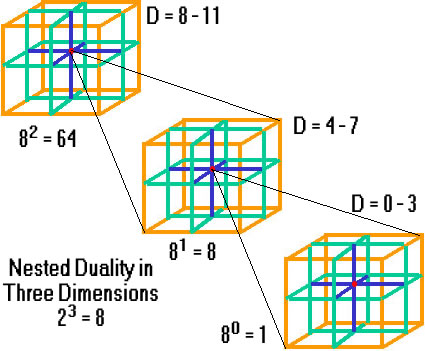
Figure 1.  Nested, N-Dimensional, Magnitudes 

So, the magnitudes of the first four dimensions, or tetraktys, form the center point of the second tetraktys, which form the center point of the next tetraktys, and so on, ad infinitum, as far as numbers go. Certainly, there would be a limit to actual physical motion combinations set by environmental constraints such as temperature and pressure. To see how this works, let’s apply the duality expansion to the second tetraktys. First, the M₁ magnitudes:

1. (8/8)⁰ = 1
2. (8/8)¹ = 1
3. (8/8)² = 1
4. (8/8)³ = 1

Next, the M₂ magnitudes (2⁴ - 2⁷):

1. (16/16)⁰ = 1 term (0 directions, or point)
2. (16/16)⁰ + (16/8)¹ = 2 terms (2 directions, or 1D line)
3. (16/16)⁰ + [(16/8)¹+ (16/8)¹] + (16/8)² = 4 terms (4 directions, or 2D area)
4. (16/16)⁰ + [(16/8)¹+ (16/8)¹ + (16/8)¹] + [(16/8)² + (16/8)² + (16/8)²] + (16/8)³ = 8 terms (8 directions, or 3D volume)

Now, the M₃ magnitudes (3⁴ - 3⁷):

1. (81/81)⁰ = 1 term (0 phases, or point)
2. (81/81)⁰ + (81/27)¹ = 2 terms (2 phases, or 1D interval)
3. (81/81)⁰ + [(81/27)¹+ (81/27)¹] + (81/27)² ] = 4 terms (4 phases, or 2D interval)
4. (81/81)⁰ + [(81/27)¹+ (81/27)¹ + (81/27)¹] + [(81/27)² + (81/27)² + (81/27)²] + (81/27)³ = 8 terms (8 phases, or 3D interval)

Finally, the M₄ magnitudes (4⁴ - 4⁷):

1. (256/256)⁰ = 1 term (0 polarities, or unipole)
2. (256/256)⁰ + (256/64)¹ = 2 terms (2 polarities, or 1D dipole)
3. (256/256)⁰ + [(256/64)¹+ (256/64)¹] + (256/64)² ] = 4 terms (4 polarities, or 2D quadrupole)
4. (256/256)⁰ + [(256/64)¹+ (256/64)¹ + (256/64)¹] + [(256/64)² + (256/64)² + (256/64)²] + (256/64)³ = 8 terms (8 polarities, or 3D octopole)

Thus, the four types of magnitudes in the CM, written as powers of 4 through 7, the four dimensions of the second tetraktys, now makes just as much sense, as those written as powers of 0 through 3, the four dimensions of the first tetraktys, even though 4, and higher, dimensions of space magnitude don’t make sense geometrically. The reason is easy to see: there are no new phenomena beyond 3 (4) dimensions. All physical magnitudes are limited to 3 (4) dimensions, but they are not limited to the same four dimensions. The first set of magnitudes in four dimensions is based on 1; the second set on 1 x 8; the third set on 8 x 8, the third set on 8 x 8 x 8, etc. In other words, on successive powers of 8,

1. 8⁰ = 1
2. 8¹ = 8
3. 8² = 64…

simply because duality, in three dimensions, produces 2³ = 8 magnitudes, at each level, as shown in figure 1. Amazing! The universe of motion is made from 8-bit bytes!

In the LRC seminar concluded two days ago, a question was asked in the virtual room about the chart of motions that we had been discussing in the meeting. I missed it, because I was saying goodbye to someone in the physical room at the time. However, the next day, listening to the recorded audio of the meeting, I finally heard it and realized that it was a very good question, and I think I will try to answer it here.

The question was, “Why do the base numbers in the rows of the chart of motion start with 1, while the column numbers in the chart start with 0? Shouldn’t the row numbers start with 0 too?” The answer is very simple, but also very enlightening. The reason the base numbers start with 1 is that the numbers of the chart aren’t arbitrary notations, but come from the mathematics of the tetraktys, the numerical expansion of dimension, which has the form:

* = 1
** = 2
*** = 3
**** = 4

Each successive row is a higher dimension, or power of numbers, starting with 0 power, which is always defined for any number as 1. However, zero is not a number and therefore can’t be raised to any power; that is, 0⁰, or 0¹, or 0², or 0³, or 0ⁿ is not a number.

On the other hand, 1 is a number. Regardless of the power we raise 1 to, it always remains 1. So 1⁰ = 1¹ = 1² = 1³ = 1ⁿ = 1. Yet, there is a spatial difference between a linear quantity of one, a square quantity of one, and a cube quantity of one, like the difference between a meter, a square meter, and a cubic meter, even though, numerically, they are all equal to 1.

Recognizing that this geometric difference, in the magnitudes of the powers of one, can have a spatial significance, leads us to conclude that it’s a magnitude difference, and since magnitudes of space don’t exist without time, we conclude that n-dimensional magnitudes are magnitudes of motion and nothing else.

It follows from this reasoning that we can generalize numbers and magnitudes, something that man has sought to do from ancient times, but has never been able to accomplish in a completely satisfactory manner. The invention of the imaginary and complex numbers, the modern approach to generalizing these two concepts, is a powerful method, but it ultimately runs out of gas in higher dimensions (or in successive rows of the tetraktys), in the form of hypercomplex numbers, because it’s an artificial, or contrived, procedure. We might call this the algebraic pathology of hypercomplex numbers.

It has long been recognized that plugging the number 2 into the tetraktys is a way to describe a sequence of algebras of real numbers, each with twice the dimension of the previous one. Producing algebras this way, known as the Cayley-Dickson construction, extends the complex numbers into hypercomplex numbers, the algebra of which is known as a Cayley-Dickson algebra. These algebras of complex and hypercomplex numbers conform to a concept of norm and conjugation, where the product of a number and the conjugate of the same number is equal to the norm of the number. The norm is simply a “size” of a vector, like the unit size of the radius in the unit circle of the complex plane, and adding the norm operation to a vector space produces a “normed vector space.” So the normed vector space used to define the U(1) Lie group, the unit circle on which we can define an infinite set of points and the complex numbers that correspond to these points, contains an infinite number of unique complex numbers that are all “size one” complex numbers, as we discussed in the seminar.

All this is just a complex way of saying that the radius of the unit circle is equal to the hypotenuse of a triangle in the circle, the sides of which are the numbers that, when plugged into the Pythagorean formula, produce a hypotenuse equal to 1. The set of the combination of numbers that will work is infinite, but it is also true that it is the operation of division that makes this possible, and, as it turns out, this operation is not possible, if we try to define more than three of these complicated vector spaces; that is, the complex numbers, forming one complex dimension (the first “normed vector space”) takes two geometric dimensions (2¹ = 2) and two numbers (z=a + bi); incrementing the complex dimension from one to two dimensions (forming the second “normed vector space”) requires two geometric planes of two dimensions (2² = 4), or four numbers (z=a+bi and z’=c+di); and one would think that incrementing the complex dimensions from two to three dimensions (forming the third “normed vector space”) requires three geometric planes of two dimensions, or six numbers (z=a+bi, z’=c+di and z”=e+fi).

However, here’s where the algebraic trouble arises in spades, because as we increase the complex dimensions to these hypercomplex numbers, the algebra of the higher normed vector space, which is so useful at one complex dimension, becomes pathological in the second and third instance. Indeed, it really becomes acute in the third such space, because for one thing, 2³ = 8, not 6. So, we really can’t use the third space as such, but have to concoct the third space out of two of the second spaces, but then this leads to other complications, and so it goes.

However, now, in light of the chart of motion, it’s easy to see the problem that is being encountered here and its solution. Instead of using the ad hoc invention of the imaginary and complex numbers to define normed vector spaces so that we can treat vectors as scalars, which have no algebraic pathology, we can, instead, recognize, following Grassmann and Clifford, that there are two interpretations of number, the quantitative and the operational interpretation.

Using the operational interpretation of number, we can define higher dimensional numbers without resorting to the concept of vectors, or vector spaces. In other words, employing the operational interpretation of number, we can obtain linear spaces of n-dimensions and the algebra of the elements in these spaces is not pathological! We do this by simply recognizing the symmetry of the tetraktys and that we can describe four dimensions of four numbers that are sixteen fundamental magnitudes. The first set of four magnitudes is:

M₁⁰ = 1⁰ = 1 potential point
M₁¹ = 1¹ = 1 potential line
M₁² = 1² = 1 potential area
M₁³ = 1³ = 1 potential volume

The second set of four magnitudes is:

M₂⁰ = 2⁰ = 1 vector point
M₂¹ = 2¹ = 1 vector line
M₂² = 2² = 1 vector area
M₂³ = 2³ = 1 vector volume

The third set of four magnitudes is:

M₃⁰ = 3⁰ = 1 interval point
M₃¹ = 3¹ = 1 interval line
M₃² = 3² = 1 interval area
M₃³ = 3³ = 1 interval volume

Finally, the fourth set of fundamental magnitudes is:

M₄⁰ = 4⁰ = 1 scalar point
M₄¹ = 4¹ = 1 scalar line
M₄² = 4² = 1 scalar area
M₄³ = 4³ = 1 scalar volume

Thus, now we can see that the “size one” of the normed vector spaces, which enables legacy physicists to do marvelous things with complex numbers, but eventually defeats them in the algebraic pathology introduced by the restriction to linear “vector” spaces that the concept of vector entails, when they are constructed with complex numbers, is easily accomplished without restricting ourselves to vectors.

In this new view, the n-dimensional “size one” magnitudes are composed of the four numbers in the tetraktys, 1, 2, 3, and 4. The “number” zero, in this number system is conspicuous by its absence, but it easily explained by our operational interpretation of number, because:

1/n, …,1/2, 1/1, 2/1, …n/1,

is equivalent to:

-n, …, -1, 0, 1, …, n.

This means that we don’t need to restrict ourselves to the infinitude between 1 and -1, which we have been availing ourselves of by means of the concept of rotation, which unites the vector concept with the interval concept of magnitude, in its complex form, but only to a limited extent.  Instead of proceeding along these lines, we can now examine n-dimensional magnitudes directly, in their natural forms.

However, how we might do this is another chapter in the continuing saga. The important point I want to make in this chapter is that the numbers 1, 2, 3, and 4, of the chart of motion magnitudes, are not arbitrarily chosen for purposes of notation, but are mathematically derived, fundamental, magnitudes of reality.

Selah. 

In discussing the concept of scalar mathematics, we’ve discussed its aspects of geometry and algebra, which is to say the relationship of numbers to geometric magnitudes in the tetraktys and the Clifford algebras, and how the scalar concepts of n-dimensional OI numbers relate to the vector concepts of complex and hypercomplex numbers (the complexes, the quaternions, and the octonions.)

In the previous post, I introduced the four numbers of the tetraktys, as four bases of motion, with four magnitudes of motion (I really messed it up too, sorry to say, but I think it makes sense now that I’ve corrected it). The motion chart, as I will call it, is extremely important in understanding the new mathematics of OI number, even though I didn’t explicitly use OI numbers to designate the bases of motion. If I had, the chart would have looked like this:

1. (1/1)⁰, (2/2)⁰, (3/3)⁰, (4/4)⁰
2. (1/1)¹, (2/2)¹, (3/3)¹, (4/4)¹
3. (1/1)², (2/2)², (3/3)², (4/4)²
4. (1/1)³, (2/2)³, (3/3)³, (4/4)³

But then the exponents of the bases aren’t OI numbers, so to be consistent, we would have to write these as OI numbers as well, like this:

1. (1/1)^1/1, (2/2)^1/1, (3/3)^1/1, (4/4)^1/1
2. (1/1)^2/1, (2/2)^2/1, (3/3)^2/1, (4/4)^2/1
3. (1/1)^3/1, (2/2)^3/1, (3/3)^3/1, (4/4)^3/1
4. (1/1)^4/1, (2/2)^4/1, (3/3)^4/1, (4/4)^4/1

Which means that we can then have another table of inverse bases with inverse dimensions, like this:

1. (1/1)^1/1, (2/2)^1/1, (3/3)^1/1, (4/4)^1/1
2. (1/1)^1/2, (2/2)^1/2, (3/3)^1/2, (4/4)^1/2
3. (1/1)^1/3, (2/2)^1/3, (3/3)^1/3, (4/4)^1/3
4. (1/1)^1/4, (2/2)^1/4, (3/3)^1/4, (4/4)^1/4

The space/time dimensions of the units of motion in the third table are t/s, not s/t, and the units are negative magnitudes, which will come in handy at some future point down the road, but would only serve to confuse things at this point, even though it shows the wonderful symmetry and completeness of the tetraktys. Nevertheless, it brings up another, very important, point that we have not directly addressed to this point: that bugaboo of ancient and modern mathematics and physics, the harmonizing of descrete versus continuous magnitudes.

In base 2 motion (vector motion), the change of position between two points means that ds/dt has a different meaning than it does in base 4 motion. This is because there is a continuum of values that ds and dt can take in vector motion, whereas in base 4 motion, there are only certain, fixed, values that ds and dt can take, because they are set by the clocks of the universe of motion, in which we assume that the magnitudes of the universe are absolute, not relative.

This seems to fly in the face of special relativity theory that maintains that time and space are not fixed, which experience has borne out, over a century of empirical tests. However, all these tests are conducted within the domain of base 2 motion, which is necessary, if we are to conduct experiments exploiting the laws of conservation and symmetry, since base 2 motion is the domain of observation of the motion of mass, or objects, where the conservation laws, based on mass, appear. Yet, clearly, the n-dimensional magnitudes of base 3 and base 4 motion are distinct in certain, important, respects, since changes in the position of massive objects are not relevant in these domains.

The ancient Greeks were never able to describe problems involving motion as speed, or velocity, because, while their mathematical language worked for problems in geometry and algebra, it was not adequate for problems of velocity. Again, the major difficulty is dealing with the notions of discrete and continuous. Base 2 speed, as a change of distance over time, depends on what interval of distance and time is referred to. If you ignore this, then Zeno’s paradox can confuse the definition of speed.

In the race of Achilles and the tortoise, if the tortoise has a head start, then Achilles can never catch it, because, in the time it takes him to close the distance, the corresponding time aspect of the tortoise’s motion is associated with a quantity of space that represents a new position, separated by a certain distance from its initial position, and, since it will always take some, finite, amount of time for Achilles to move the distance that separates them, no matter how small the distance, the tortise will always have that much time to move a little further away.

This is just another way of saying that space does not exist independently of its association with time in motion. We cannot measure space without time, or time without space; regardless of the magnitude of the ratio of space/time, it always has two, reciprocal, aspects. The only reason that Achilles, can in fact, catch up with the tortoise, and surpass it, is found in the speed of the tortoise, which in real life, is fixed. The speed of the tortoise in Zeno’s paradox is actually changing, because as the interval of time gets smaller and smaller, there’s always an interval of space associated with it by definiton, regardless of how small it is. Thus, the speed of the tortoise, in the paradox, reaches the speed of light, when the interval of time, and the interval of space reach the natural units of space and time.

At that point, neither Achilles nor the tortoise can go any faster, and the distance between their locations becomes absolute. So, we conclude that, while the time and distance separating two locations is infinitely divisable, the ratio of time and distance, as the reciprocal unit change of space per unit change of time, is limited to a natural unit value, one natural unit of space, per natural unit of time, the speed of light.

However, in LST physics, the fact that both distance and time, as quantities between two locations, are infinitely divisable, as Zeno’s paradox seems to show,  this idea is used to define velocity, not in the reciprocal limit of unity, but in the quantitative limit of zero; that is, velocity is defined “in the limit” of delta s over delta t, when delta t gets “vanishingly small.”  It is written as

v = lim (Δt -> 0) Δs/Δt,

where the symbols in the parentheses are usually written under the letters “lim,” which I can’t do in html.  This means that space, for purposes of base 2 motion calculations, is defined as

Δs = v Δt,

provided that the velocity does not change during the quantity Δt, which means Δt has to be very close to zero, or “vanishingly small.”  This way of thinking, derives from the fact that base 2 motion can be any value at any time, so, in order to define it precisely enough, it is necessary to “pin it down” like this, to the smallest possible interval of time.  Thus, the mathematics of motion, must become the mathematics of change first and foremost, and the ancient Greeks just didn’t have the required mathematical concepts. 

The mathematics of change, called the differential calculus, came from Newton and Leibniz, and forms the basis of LST physics. The concept of quantity, in the definition of motion, Δs/Δt, where Δt is zero, but not really zero, that is, it is infintesimally small, was the beginning of the use of a principle in LST physics called the “to a good approximation” principle.  It is something that the ancient Greeks would have found abhorent, and it has come back to haunt modern physics too, in the end.

However, it works, and to the degree that it works, it can support technological applications that change society radically. So, even though the philosophers object, the practicioners are delighted.  Yet, when the practicioners want more from our understanding of nature, the practicality of “to a good approximation,” becomes a barrier to further progress, and it’s at that point that we must turn to the philosophers for help.  “What’s wrong with our understanding?” we want to know, “Why can’t we understand what mass is and where it comes from?  Why don’t we have a better theory of charge? Why can’t we understand the common origins of electrical, magnetic, and gravitational forces?”

Well, at the LRC, we believe that we can answer these kinds of questions, if we redefine motion, which means we need a better understanding of the nature of space and time. To define space in terms of the product of velocity and an infinitesimal interval of time is not good enough, even though it works “to a good approximation.”   Now, with the knowledge of base 3 and base 4 motion of the tetraktys, as seen in the motion chart, we can begin to see that we can’t use the concepts of differential calculus, as it was developed for applications of base 2 motion, which depends on an object’s change of position.  We need a different calculus in dealing with base 3 and base 4 motion, because these motions are not based on arbitrary changes of position over time, but on fixed changes of interval and size over time.