The New Mathematics
Mathematics for Dummies
 Doug
Doug
 Post a Comment
Mathematics has a life of it’s own and has grown into an incredible array of complexity, layered like sediment in an ancient lake bed, over century upon century, by mathematicians. However, as Hestenes points out, the development of mathematics useful for physics is not the responsibility of mathematicians, but physicists, and history has shown that this line of mathematical development has generally resulted from successful attacks on physical challenges.
Today’s crisis in theoretical physics, precipitated by contradictions at the fundamental level, with respect to the discrete vs. continuum characteristics of nature, is generating new mathematics, but it is producing mathematics that is extremely complex, elaborate and baroque and not necessarily useful for physics, yet (string theory). Maybe this is because today’s physics has become so mathematical, that the mathematical physicists are more interested in researching the principles of mathematics than they are in researching the principles of theoretical physics.
Here at the LRC, we work with a brand new principle of physics, called scalar motion, and a “new” principle of mathematics, the operational interpretation of number, in an effort to form a brand new science, based on these principles, called scalar science. To many investigators of Larson’s Reciprocal System theory (RSt), which he developed from his Reciprocal System of Physical Theory (RST), the lack of an appropriate mathematical formalism is painfully evident. Yet, at the LRC, we have discovered that Larson provided the fundamental insight for what we now are calling scalar mathematics and that it is much more than a modern mathematical formalism; It is the discovery of a fundamental principle of mathematics that is founded on the same underlying reality as is the fundamental principle of motion - the principle of reciprocity.
In the modern LST community, the major principle of mathematics guiding the research of theoretical physics is symmetry, and the mathematical formalism upon which it is based is called group, and group representation, theory. Specifically, it is a special type of group, called a Lie (Lee) group that is most useful to the physicists. In fact, it’s a special type of Lie group, called a simple Lie group that the LST community is mostly interested in, and within these, it is the complex ones that they use most, and especially the ones in compact real form.
Hence, when authors refer to Lie groups, and their associated Lie algebras, the term has to be qualified, because of the complexity of the subject. For instance, one could be concentrating on “compact real forms of complex simple Lie groups” and refer to these groups as Lie groups for brevity, but obviously the term is highly qualified. Needless to say, however, the complexity involved in the use of these concepts is tremendous and very daunting for neophytes, wanting to learn how to study physics, based on the simple principles of symmetry.
Fortunately, the principle of reciprocity is the epitome of symmetry. Hence, at the LRC, mastery of Lie groups and Lie algebras is not a prerequisite to study the role of symmetry in physics. The only prerequisite here is a thorough understanding of the principle of reciprocity. Consequently, we begin at the beginning in mathematics and physics, with the fundamental definitions of units, dimensions, and directions in defining the magnitudes of motion, and the spaces of geometry, with numbers.
Nevertheless, we can, and many times do, refer to LST concepts to connect the new with the old, because it’s important to understand that scalar science does not replace vector science, but is actually an extension of it. In our effort to demonstrate this, and to clarify the relation between scalar science and vector science, we focus on the ancient Greek concept of the tetraktys, or the first four numbers, 1, 2, 3, and 4, which, to the ancients (not only the Greeks), contained the mystery of the cosmos.
It is in the tetraktys that we clearly understand the connection of geometrical units and numbers, and have discussed the work of Hestenes a great deal, in this connection, because he was the first to emphasize the importance of Clifford algebras as geometric algebras (GA), and how they can be used to great advantage in the study of physics. In fact, it turns out that 3D Clifford algebra is the Lie algebra of physical space, and since Lie algebra is the infinitesimal group of the Lie group, or elements of the Lie algebra are elements of the groups that are “infinitesimally close” to the identity of the group, every field and geometry in physics can be described by Clifford valued forms (see: Garrett’s tutorial on Physics Forums).
However, it’s important to understand that the study of symmetry in this way necessarily includes the concept of rotation in connection with the dimensions of geometry, and the concept of the smooth manifolds of topology, which increases the complexity of the subject immensely. This is especially so, given that the concept of rotation is obtained through the ad hoc invention of the imaginary number. While GA replaces the concept of rotation in terms of complex and hypercomplex numbers, with a much more compact, intuitive, concept of rotation, which helps somewhat, it doesn’t simplify the complexity of using differential forms and vectors to describe the symmetries of interest, the symmetries of the standard model of particle physics, SU(3)x(SU(2)x(U(1).
Fortunately, however, the knowledge of scalar mathematics is shedding a good deal of light on the subject and clarifying the concepts involved. We’ve seen how the operational interpretation of rational numbers (OI) makes it possible to define two “directions” of numbers (positive and negative) without recourse to the ad hoc invention of the imaginary number, i, where -1 is defined as its square. With the OI, we define negative numbers with the principle of reciprocity instead. If we consider the three dimensions of the universe of motion in light of the OI, instead of i, we see a remarkable clarification of what n-dimensional numbers actually are. Indeed, we can again see why the tetraktys is so central.
Figure 1, below, shows the four numbers of the tetraktys in terms of dimensions of motion and dimensions of spaces. We recall the words of Newton, who pointed out that principles upon which the spaces of geometry are defined, are not principles of geometry, but come from “without,” from another dimension, if you will. In figure 1, we see that these principles are actually the three dimensions of the tetraktys, 0, 1, 2, and 3.
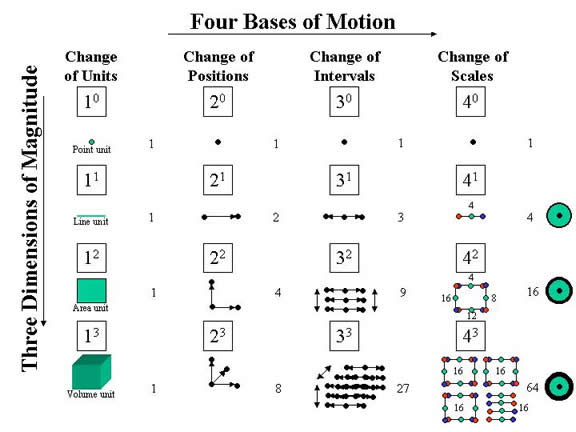
Figure 1. The Four Dimensions of Motion
In the first column of the chart in figure 1, we see the first dimension of motion, or what we will call the first base of four bases of motion, to distinguish them from the four dimensions of magnitude. This is the number 1 of the tetraktys, as it increases in geometric dimension, row by row, corresponding to the unit point, unit length, unit area, and unit volume spaces, or distance measures, of Euclidean geometry. Of course, 1 is 1/1 in the OI, and, as a scalar number, can be raised to any power, (1/1)n = 1, but its geometric dimensions are: 1, 1x1, and 1x1x1, the unit line, the unit plane, and the unit volume, the “right lines and circles” of geometry, to use Newton’s phrase.
However, these units of space, can only be created by motion, and the first dimension of magnitude of the first base of motion is zero, or no motion. Hence, these units are the potential spaces of geometry, which must be created by magnitudes of motion, a reciprocal relation of space and time.
The second column of the chart shows the second base of motion, or the number 2 of the tetraktys, as it increases in magnitude dimension, row by row, corresponding to the change of position between two points. Again, 2, to the zero power of magnitude, is no motion, which is equivalent to the number one, or a geometric point, but the three non-zero magnitude dimensions are: 2, 2x2, and 2x2x2, representing the separation of two points in magnitude dimension 1, the separation of four points in magnitude dimension 2, and the separation of eight points in magnitude dimension 3, corresponding to the magnitude dimensions of this motion required to define the unit magnitude spaces of column one; that is, with the base 2 motion, we can define a line in one dimension of magnitude, by separating two points; We can define an area in two dimensions of magnitude, with this motion, by separating two points in two orthogonal directions (22), and we can define a volume in three dimensions of magnitude, with this motion, by separating two points in three orthogonal directions (23).
However, notice that all the units of space defined by base 2 motion are necessarily positive units. This means that the numbers constructing the spaces with this motion are all positive. If it is unit distance we are considering, then we can produce the unit line, the unit area and the unit volume, as real objects, but since space is not an independent entity, both space and time are required to construct the spaces. In this case, the motion that separates the points must be in one direction at a time, so that to define an area requires two instances of the motion, and to describe a volume requires three instances of the motion. Moreover, a rotation of ninety degrees must separate each instance of the motion; that is, without the concept of rotation, we cannot transform the motion from one dimension to the next. Does this mean we need the imaginary number?
The answer is obviously no, in this case, because all the spaces to be defined are positive. All that we need is two rotations to orthogonal angles, which are defined by the unit spaces of column one. If we define the distance in one direction, with the number x/1, and the distance in an orthogonal direction with the number y/1, and the distance in a direction orthogonal to both the preceding directions with the number z/1, we can define the three required spaces. We conclude, then, that geometric orthogonality is achieved in base 2 motion through rotation.
The next base of motion is the third base, base 3 motion, corresponding to the number 3 of the tetraktys. Again, the zero geometric dimension of this motion is no motion, which is equivalent to the point. However, the first dimension of magnitude, of the base 3 motion, requires a separation of three points; the second, requires a separation of nine points, and the third dimension of magnitude requires a separation of twenty-seven points, or 3, 3x3, and 3x3x3.
Since base 3 motion defines a line with three points, the distance separating the points is constructed by two, simultaneous motions in opposite directions with respect to the center point. Since the inverse of x/1, y/1, and z/1, is 1/x, 1/y, and 1/z, we can see that when x, y, and z = 1, then there is no way to distinguish any of these numbers from any other. In other words, they are all equal to 1/1, when x, y, and z = 1, so this value forms the intersection of all non-unit values of x, y, and z. In the case of one geometric dimension, increasing the values of x, from 1 to 1+ n, increases the distance from 1/1 in both directions simultaneously. The same for values of y and z.
Consequently, if the first instance of base 3 motion creates a line between the two opposing values of x, by virtue of a linear expansion between three points, then a subsequent expansion in the y or z direction will expand the initial linear expansion in the orthogonal direction in two opposing directions. This creates an area consisting of nine points (an area of three, three-point, lines). A final expansion in the remaining orthogonal direction, produces the required volume consisting of twenty-seven points (a volume of three, three-line, planes).
Notice, however, that in the case of base 3 motion, the concept of rotation through an angle is not implicit. The rotation of a line along its longitudinal axis is not defined in this motion base. So, we conclude that the transformation from one dimension of magnitude to the next does not require rotation in base 3 motion. We will come back to consider the implications of this fact below, but for now let’s just be sure to note that the spaces of this motion, produced by a change of interval, or we might say by an expansion of an interval, involves two, opposed directions, a negative and a positive direction, with respect to the center. However, just as stretching a rubber band in two, opposite, directions does not make half of it positive and half of it negative, so too in this case. The n-dimensional spaces defined by base 3 motion are all positive. This is an important observation, the discussion of which we will also defer until later.
Finally, the fourth column of motion, base 4 motion, is the row by row geometric expansion of the last number of the tetraktys, the number four. As indicated in figure 1, whereas, base 2 motion is defined by change of position, and base 3 motion is defined by change of interval, base 4 motion is defined by change of scale. In the previous dimensions of motion, we indicate change of position in one direction by adding units of distance to the initial value of 1 unit, but with the OI, the value of 1/1 replaces zero, which is not a number. Hence the actual distance magnitude is a displacement from 1, not zero. For example,
x = 1/1 = 0,
because there is no difference between the denominator value, and the numerator value; that is, there is zero displacement between the two aspects of the number. The displacement, or the value of the relation of the numbers defines the magnitude, not the value of the numbers themselves (see: John Baez’s discussion of torsors). Thus,
x = 2/1 = 1; 2x = 3/1 = 2; nx = (n+1)/1 = (n-1), when n > 1.
Of course, the inverse of these magnitudes gives us the values of negative directions (remember, not negative spaces, but negative direction):
-x = 1/2 = -1; -2x = 1/3 = -2; -nx = 1/(n+1) = -(n-1), when n> 1.
In base 2 motion, there is motion in only one direction (positive). In base 3 motion, there is motion in both the positive and negative directions simultaneously, as shown in figure 1. Now, in both of these case, the motion defines the magnitude, by moving an object; that is, the units of x, y, and z are units of distance produced by the change of position of an object (separation of two points) over time, or the expansion of an interval (separation of three points), over time. However, in the case of base 4 motion, no object is involved in the motion, and the units of distance and time are always unit distance and time, so while it’s related to base 2 and 3 motion, base 4 motion is also very different.
Scalar motion is a measure of the progression of space and time, where space progresses just as uniformly and eternally as time does. Discrete units of this motion are created when the progression of one or the other of its two reciprocal aspects is continuously increasing and decreasing between two successive values, such as n and (n - 1). Thus, the alternating aspect increases at half the rate as the non-alternating aspect, producing a displacement in the rates of increase of the two progressing aspects. Consequently, the space/time ratio, or velocity, of the motion, in a displaced unit, never changes, but the scale of the displacement does change; that is, just as the ratio of 50/100, or 25/50, or 5/10 is all the same ratio, namely 1/2, the scale of 50/100 is very different than the scale of 1/2.
Since this is the case, what we are measuring in base 4 motion is units of velocity, and inverse velocity, not units of space. The unit of space that participates in the calculation of the velocity, is three-dimensional, because an increase/decrease in volume is the scalar magnitude in a 3D universe. It is the increase of the scalar point to the 3D pseudoscalar volume, as shown in column four of the chart in figure 1. Again, the first dimension of magnitude of the number, the zero dimension, is not detectable as motion, because no displacement can occur in a zero-dimensional system, and, like all the other numbers before it, 40 motion is equivalent to the point.
However, with one dimension of magnitude, two displacements can be formed, as before, where either the value of the denominator or the value of the numerator, becomes greater than its reciprocal. Nevertheless, with no object to define the motion, the values of denominator or numerator cannot can be increased independently, like the numbers on an odometer. Only when the alternating increase/decrease pattern in the progression of one of the two aspects of the unit motion occurs, at a given point in the progression, can the 1/2 (one negative unit), or 2/1 (one positive unit), displacement occur. Therefore, the minimum number of progression units over which an alternating pattern can occur is two units. In other words, if the space aspect of
ds/dt = 2/2,
is alternating between increase and decrease, then its rate of increase will be reduced to every other unit, while the time unit continues to increase with every unit of progression. This conditions alters the increasing space/time ratio to
ds/dt = 1/2,
or, in the case of the alternating progression of the time aspect, to
dt/ds = 1/2,
representing a negative and positive unit of motion, when the dt/ds unit is inverted to ds/dt = 2/1. Combining these two units, then, is essentially combining two units of 2/2 progression, which is a total of 2/2 + 2/2 = 4/4 units of progression. However, one unit of space in the negative unit, and one unit of time in the positive unit, the decreasing units, can be combined separately to provide a numerically correct equation of the motion:
ds/dt = 1/2 + 1/1 + 2/1 = 4/4 num,
where num is short for natural units of motion. Notice the similarity of displacement in this motion and the displacement of the base 3 motion with 1 dimension of magnitude. The difference is that the displacement of the base 4 motion is not one unit of distance expansion in the negative direction, but one unit difference in the progression rate of space/time; that is, in the ds/dt = 1/2 value of base 4 motion, the progression rates of space and time are displaced so that the rate of time progression is twice the rate of space progression, over two units of progression. In effect, this displaced velocity is one half the unit velocity of the undisplaced progression, where the rates of the space and time progressions are equal.
Thus, while the two velocities (ds/dt = 1/2 and ds/dt = 2/1) are equal in terms of their displacement from 1/1, in their respective “directions,” they are unequal in terms of their velocities, as the velocity of 2/1 is four times as fast as the velocity of 1/2 (2/.5 = 4). Note, however, that the velocities are actually one cycle of increase/decrease values, or frequencies. The important thing to understand is that the “distance” between the two frequencies is one unit of magnitude in one “direction” and one unit of magnitude in the opposite “direction,” relative to the unit value in the center, which is isomorphic to a one-dimensional line of magnitude four.
Thus, in the next row, with 2 dimensional magnitude, the value of the “area” magnitude is 4x4, or four times the “line” magnitude, which can be illustrated by arranging four “lines” of magnitude as four lines in a square, even though, no rotation of the “line” is conceivable. Likewise, with 3 dimensional magnitude, the 4x4x4 magnitude of motion can be arranged to form a cube, even though this is just an equivalent to the total 1D magnitudes of motion contained in the unit 3D magnitude.
What this shows, then, besides the unity of dimensions of numbers and the magnitudes of geometry, is that the symmetry of motion can be dramatically demonstrated, without the use of imaginary numbers, or even the concept of rotation. That is to say, we can see now that rotation has only a limited role to play in the total picture of motion. It is only applicable to the base 2 motion of the tetraktys, while the real key to understanding symmetry, the principle of reciprocity, is orders of magnitude more powerful.
Later, we will discuss how these dimensions of motions form groups, and what that means in terms of group theory, but that’s all for now folks.
Update: 8 Dec 06 - I’ve edited the text to correct errors in references to the various bases of motion. I appologize for the confusion in the original text, which was caused by confusing dimensions of magnitude with dimensions of motion. Changing the terminology helps to keep the concepts clearer and to avoid mixing up the numbers as I did. I hope it’s easier to understand now.
Speaking of New Math
Peter Woit’s current entry is entitled King of Infinite Space, and it’s about H.S.M. Coxeter and the new biography about him, by Siobhan Roberts. I’m definitely going to read Roberts’ book. I hope she gives the correct pronunciation of his name in it. If not, can someone here give me a clue as to how to pronounce his name that doesn’t sound obscene?
I’d also like to observe that, unlike Peter, Danny, and others who have commented on Peter’s post, I had no interest in these things as a child. My interests were in sports (marbles, tetherball, kickball, softball, basketball, football) and airplanes. I loved aviation, and daydreamed about flying in middle school, when these guys were thinking of polytopes!
I vaguely remember being taught something about sets, I think, but my seventh grade algebra teacher told me that I probably ought not to consider a career in mathematics. I sort of had a mild version of the “crying jags” over the meaning of the “two roots” of the number one, and the necessity for the imaginary number it conjured up, only my problem wasn’t trying to imagine negative cabbages, but just trying to understand what the statement of the problem meant. I couldn’t understand how to relate the concepts of “roots,” the radical, and imaginary numbers, and do it all within the confines of a 7th grade class period.
Now I realize how little foundation for understanding numbers, magnitudes, and the operations that relate them, I actually had. So, while those really smart guys were having fun with all this, we dummies were so lost and perplexed that we grew to hate the stuff.
Now, with a more mature perspective, I want to understand what I didn’t understand as a child, but it’s tough going. The experience of learning that Coxeter’s career was sort of a counter-revolutionary one, viz-a-viz the new math Bourbaki, is kind of like having to have someone explain a joke to you. It helps you understand what the joke was about, but it doesn’t make you laugh, and you still feel left out in a sense.
I’m really a late comer. I didn’t even know about Coxeter, or the Bourbaki, until Peter posted his experiences with the man’s ideas. Now, thanks to the Internet, I can see that he is credited with saving the subject of geometry from being completely abandoned by educators, who were convinced that geometry was nothing but an impediment to learning algebra. The Bourbaki were a group of French mathematicians whose ralling cry was Jean Dieudonne’s rant “Down with Euclid, death to the triangles!” (the French!!!). As Roberts explains:
In the 1930s, a secret society of crème de la crème French mathematicians sat in a Parisian café and devised an outlandish prank: They invented a mathematician by the name of Nicolas Bourbaki and decided to write under this nom de plume, publishing an encyclopedic treatise that aimed to restructure the discipline of mathematics axiom by axiom. Mathematical folklore has it that, for a time, the international mathematical community was duped; papers appeared by Nicolas Bourbaki, yet no one knew this man who never turned up at conferences as promised.
Writing in the Boston Globe, Roberts gives us the motivation for her book:
Crying `Death to Triangles!’ a generation of mathematicians tried to eliminate geometry in favor of algebra. Were it not for Donald Coxeter, they might have succeeded…Through his lifelong work as geometry’s apostle, Coxeter, who died in 2003 at 96…, became known by his followers around the world as “the man who saved geometry” in a mathematical era characterized by all things algebraic, abstract, and austere.
I guess I’ll have to read the book to learn the details of this “New Math” melodrama, but Peter gives us a flavor of what it entailed from his personal experience:
One theme of [Roberts’] book is to set Coxeter, as an exemplar of the intuitive, visual and geometric part of mathematics, up against Bourbaki, exemplifying the formal, abstract and algebraic. Bourbaki is blamed for the New Math, and I certainly remember being subjected by the French school system in the late sixties to an experimental math curriculum devoted to things like set theory and injective and surjective mappings. On the other hand, I also remember a couple years later in the U.S. having to sit through a year-long course devoted to extraordinarily boring facts about triangles, giving me a definite sympathy for the Bourbaki rallying cry of “A bas Euclide! Mort aux triangles!”. To this day, both of these seem to me like thoroughly worthless things to be teaching young students.
Here’s where it starts to get interesting, because, as we see over and over again, the real behind-the-scenes struggle is between the discrete and the continuous. Peter makes a comment that reveals this, when he writes:
Actually Bourbaki and Coxeter ended up having a lot in common. They both pretty much ignored modern differential geometry, that part of mathematics that has turned out to be the fundamental underpinning of modern particle physics and general relativity. Coxeter’s most important work probably was the notion of a Coxeter group, which turns out to be a crucial algebraic construction, and ended up being a main topic in some of the later Bourbaki textbooks. A Coxeter group is a certain kind of group generated by reflections, and Weyl groups are important examples. Coxeter first defined and studied them back in the 1930s, part of which he spent in Princeton. Weyl was there at the same time giving lectures on Lie groups, and used Coxeter’s work in his analysis of root systems and Weyl groups.
Coxeter groups and associated Coxeter graphs pop up unexpectedly in all sorts of mathematical problems, and Roberts quotes many mathematicians (including Ravi Vakil, Michael Atiyah and Edward Witten) on the topic of their significance.
Peter’s complaint that “They both pretty much ignored modern differential geometry, that part of mathematics that has turned out to be the fundamental underpinning of modern particle physics and general relativity,” is a complaint that the mathematics of discrete principles of symmetry, such as Coxeter’s groups, seem to have no relevance to physics. As he explained earlier in his comment:
Coxeter’s main interest was in “classical” geometry, the geometry of figures in two and three dimensional space and he wrote a very popular and influential college-level textbook on the subject, Introduction to Geometry. Much of this subject can be thought of as group theory, thinking of these figures in terms of their discrete symmetry groups. This subject has always kind of left me cold, perhaps mainly because these groups play little role in the kind of physics I’ve been interested in, where what is important are continuous Lie groups, both finite and infinite-dimensional, not the kind of 0-dimensional discrete groups that Coxeter mostly investigated.
Of course, zero-dimensional, vectorial, magnitudes, which are really 1, 2 and 3 “dimensional,” scalar, magnitudes, is what we are all about here at the LRC. The idea of abstract algebra, based on group theory, is all the rage in physics today, but I think the difference between the n-dimensional, continuous, Lie groups and the zero-dimensional, discrete, Lie groups that Coxexter championed, may have more to do with today’s fundamental crises in theoretical physics than people realize.
The continuous Lie groups have to do with rotations, and the continuum of smooth manifolds, with the associated connections, covers, fiber bundles, etc, which wouldn’t be possible without imaginary numbers, and the complex and hypercomplex numbers that they make possible, even though these concepts have their equivalents in the three-dimensional Clifford algebra, which treats rotations in a more efficient manner than can be done with complex and hypercomplex numbers.
However, the key aspect to understand in all this is the role of rotation in the concept of higher dimensions. Is rotation, and all the baggage it brings with it, really necessary to define magnitudes of higher dimensions, or is there another way, a way that might lead to resolving the continuum - discrete dilemma that is perplexing modern theoretical physics?
I’ll start discussing this next.
Bott Periodicity Theorem
In the eighth post copied from the BAUT forum thread (see the previous 10 posts), I briefly explained how the Bott Periodicty theorem is easily seen in the Reciprocal System of Mathematics (RSM), used in the scalar science of the LRC. However, I would like to demonstrate it more completely by focusing on the theorem’s role in current legacy system (LST) research, to contrast the use of the math of the two systems.
We can start with the Wikipedia article on Bott Periodicty, recalling that what the theorem says in short is that there is no new phenomena beyond three dimensions. This implies then that the concept of 10 dimensions, which is the foundation of string theory, has to cope in some manner with the theorem. The Wikipedia article states:
In mathematics, the Bott periodicity theorem is a result from homotopy theory discovered by Raoul Bott during the latter part of the 1950s, which proved to be of foundational significance for much further research, in particular in K-theory of stable complex vector bundles, as well as the stable homotopy groups of spheres. Bott periodicity can be formulated in numerous ways, with the periodicity in question always appearing as a period 2 phenomenon, with respect to dimension, for the theory associated to the unitary group. See for example topological K-theory.
Now, homotopy theory has to do with functions in topology, and K-theory has to do with topology, as a branch of algebraic K-theory, which is used to study topological spaces. I seem to remember reading Michael Atiyah, the originator of the Index theorem, stating that it is used to find the number of solutions to a system of differential equations in a given algebraic space, which can be useful in finding the actual solutions themselves, something like knowing that there are 180 degrees in the angles of a triangle is helpful in finding the value of a given angle that otherwise would be much more difficult to do.
With the index theorem, the shape, or the topology, of the space under study provides the clues needed to get at the solutions to differential equations that the vectorial system of physical theory requires. What Atiyah (and Singer) did, was to use K-theory to demonstrate that the index could be described topologically. This was huge and led to the popular connection between topology and theoretical physics. Indeed, from what I understand, it was the mathematical methods derived from the index theorem that enabled Witten to make his significant contribution to string theory.
Anyway, the Wikipedia article on algebraic topology states:
The goal is to take topological spaces and further categorize or classify them. An older name for the subject was combinatorial topology, implying an emphasis on how a space X was constructed from simpler ones. The basic method now applied in algebraic topology is to investigate spaces via algebraic invariants, by mapping them, for example, to groups which have a great deal of manageable structure in a way that respects the relation of homeomorphism of spaces. This allows one to recast statements about topological spaces into statements about groups, which are often easier to prove.
Of course, it is the study of groups, in group theory, that connects all this to modern physics, especially to string theory. I’ve written several times about the connection of the octonions to modern physics and their connection through the periodicity theorem that John Baez finds so mysterious (Period Eight, or Bott Periodicity, Strikes Again!), but back in May of 2000, Dr. Rick Ye, gave a talk at what is now the KITP in Santa Barbara entitled “The Bott periodicity theorem,” where he explains that there are various ways to state the theorem in terms of the topological language of groups, and later he goes through proofs of these, but, after he explains three versions of this period eight theorem, he talks about why it is important, and gives four reasons:
- It is the fundamental structure theorem for K-theory, which enables computations to be made in homotopy structure.
- Homotopy structure of the unitary groups is the cornerstone for everything based on these groups (standard model).
- It leads very quickly to Thom isomorphism and then to the Atiyah-Singer Index theorem.
- It’s needed for D-branes!
The relation between the period eight of Bott periodicity, K-theory, mathematical groups, Index theorem, and D-branes in string theory, seems to be simply that it maps the D-branes of different dimension, as seen through the eyes of vectorial physics, using vectorial spaces, and the system of differential equations clothed in the language of the shapes of spaces, or topology.
It’s all very complicated and involved. However, what we have discovered in scalar physics is that vectorial physics appears to be the wrong system for describing the internal degrees of freedom of physical entities, and the vectorial mathematics of differential equations is the wrong language for investigation of these properties, and the vectorial geometry of vectorial motion is the wrong geometry. Thus, the science of using complex concepts of topology, connected to complex concepts of groups, connected to complex systems of differential equations, are simply inappropriate for calculating the properties of these entities. Physicists may be able to get there from here, eventually, or not, but why beat our heads against the wall? It appears that scalar science offers a much simpler route to understanding these properties.
Take Bott periodicty for instance. When viewed from the standpoint of scalar mathematics, this phenomenon becomes trivially simple to comprehend. Recall that the first reciprocal number (RN) is
ds/dt = (1/2 + 1/1 + 2/1) = 4/4 nm,
where nm is natural units of motion. As explained previously, this equation exploits the operational interpretation of numbers of the RSM to express the motion combination of the two unit speed-displacements of the RST, which we have called the SUDR and TUDR, into one composite unit, designated as S|T. The RN is a three-dimensional number that can express the period eight phenomenon in terms of a power expansion, by first showing that the quadratic expansion of the RN is isomorphic to the binomial expansion, given the OI of RSM:
•20|40 (1/1) = 1/1 nm
•21|41 (1/2 + 1/1 + 2/1) = 4/4 nm
•22|42 (4/8 + 4/4 + 8/4) = 16/16 nm
•23|43 (16/32 + 16/16 + 32/16) = 64/64 nm
•20|40 (1/1) = 1/1•21|41 (1/2 + 1/1 + 2/1)1 = 4/4•22|42 (1/2 + 1/1 + 2/1)2 = (4/4)2 = 16/16•23|43 (1/2 + 1/1 + 2/1)3 = (4/4)3 = 64/64•24|44 (1/1) = (4/4)4 = 256/256•25|45 (1/2 + 1/1 + 2/1)5 = (4/4)5 = 1024/1024•26|46 (1/2 + 1/1 + 2/1)6 = (4/4)6 = 4096/4096•27|47 (1/2 + 1/1 + 2/1)7 = (4/4)7 = 16384/16384•28|48 (1/1) = (4/4)8 = 65536/65536•29|49 (1/2 + 1/1 + 2/1)9 = (4/4)9 = 262144/262144•210|410 (1/2 + 1/1 + 2/1)10 = (4/4)10 = 1048576/1048576•211|411 (1/2 + 1/1 + 2/1)11 = (4/4)11 = 4194304/4194304
This shows how each dimension, n, can be expressed as a power of the first RN, or 2n ~ 4n = RNn. Finally,
•20|40 (1/1) = 1/1•21|41 (1/2 + 1/1 + 2/1)1 = (2/2)2•22|42 (1/2 + 1/1 + 2/1)2 = (4/4)2 = 16/16•23|43 (1/2 + 1/1 + 2/1)3 = (8/8)2 = (1*8/1*8)2 = 64/64
•24|44 (1/1) = (4/4)4 = (16/16)2 = (2*8/2*8)2 = 256/256•25|45 (1/2 + 1/1 + 2/1)5 = (32/32)2 = (4*8/4*8)2 = 1024/1024•26|46 (1/2 + 1/1 + 2/1)6 = (64/64)2 = (8*8/8*8)2 = 4096/4096•27|47 (1/2 + 1/1 + 2/1)7 = (128/128)2 = (16*8/16*8)2 = 16384/16384
•28|48 (1/1) = = (4/4)8 = (256/256)2 = (32*8/32*8)2 = 65536/65536•29|49 (1/2 + 1/1 + 2/1)9 = (512/512)2 = (64*8/64*8)2 = 262144/262144•210|410 (1/2 + 1/1 + 2/1)10 = (1024/1024)2 = (128*8/128*8)2 = 1048576/1048576•211|411 (1/2 + 1/1 + 2/1)11 = (2048/2048)2 = (256*8/256*8)2 = 4194304/4194304
shows why the period eight is fundamental to higher dimensional numbers. And we have always thought that the 8 bit byte was a necessary, but rather arbitrary, basis for the binary language of computers!
Anyway, the bottom line here is that because we don’t need the systems of differential equations upon which vectorial physics is based, we obviously don’t need all that complex homotopy stuff either. Evidently, all that we need is some good computer engineers! LOL
I was watching an interview of Bill Gates on cable last night. I wonder how intrigued he would be with this? It really doesn’t matter, but he does have the economic clout to gather some really competent mountain climbers at the foot of this mountain, a mountain that the amatuer Larson discovered, but that the professionals like Lee Smolin should prepare to climb (to use his own metaphor).
Alas, we probably can’t even get Smolin’s attention, let alone Gate’s attention. Pity.
Tenth Post in the BAUT RST Forum
The tenth post in the BAUT forum follows. These posts are a continuation of the RST thread in the “Against the Mainstream” forum of BAUT.
+++++++++++++++++++++++++++++++++++++++++++++++++++++++++++++++++++++++++++++
The first question that usually occurs to those studying Larson’s works is, “What causes these ‘direction’ reversals?” Larson’s answer is that no mechanism is required to be identified in this case, because it lies outside the scope of the system (related to Godel’s incompleteness theorem I think.) In other words, in order for the system to be applied at all, n units of one aspect must be associated with 1 unit of its inverse aspect, and the only way that this is possible is for the scalar “direction” of the progression of one aspect or the other, to “oscillate;” that is, it must alternately increase/decrease in value, which is the only sense in which a scalar value can “oscillate.”
Thus, if, at some given space/time location in the progression, the scalar value of one aspect is alternately increasing/decreasing, while the inverse aspect at that location continues to increase normally, the space/time progression ratio at that location will not be 1/1, but 1/2 or 2/1. This result can be easily plotted on a world line chart as shown in figure 1 below, where the scalar increase of time is plotted on the vertical axis and the scalar increase of space is plotted on the horizontal axis.
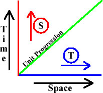
Clearly, if the unit, 1/1, space/time progression is plotted on this chart, it will fall along the green line, where ds/dt progresses as:
1/1, 2/2, 3/3, …, n/n.
However, if the space aspect of the progression, at a given location, say at 3/3, is alternating between 2 and 3 continuously, the uniform increase in the progression of space at that location will effectively stop, while the uniform increase of the time aspect at that location will continue to increase normally.
Notice that the space progression doesn’t actually stop, as this would be impossible, but since each increasing step is offset by a decreasing step, the forward progress effectively ceases, as it would if a marching soldier took a step backward every other step. Thus, the spatial location at this point in the progression is fixed by the space “oscillation,” while the space/time progression ratio of the location is ds/dt = 1/2, because the space progression is now confined to one unit (3-2 = 1), and within that unit only half of the total units of progression are increases, the other half are decreases. This location is indicated on the chart by the circled red S, and its inverse, caused by an equivalent “oscillation” in the time aspect, is indicated by the circled blue T.
Consequently, the world line for the red S is plotted as a vertical red line, since only its vertical component (time) uniformly increases. Likewise, the world line for the Blue T is plotted as a horizontal blue line, since only its horizontal component (space) uniformly increases. In other words, discrete units of space motion, albeit stationary in space, are created by space “direction” reversals, while discrete units of time motion, albeit stationary in time, are created by time “direction” reversals.
So far, the logical consequences of the system are clearly evident, or what more formally is referred to as apodictic; that is, they are demonstrably true, or incontrovertible. However, when Larson arrived at this point in his development, he had to find way in which n units of one aspect of the progression are associated with 1 unit of its inverse aspect, where n is not fixed at 2. To do this he concluded that another “direction” reversal pattern is possible, where the alternating increase/decrease in one aspect of the space/time progression only continues for a period of time (or space). When this period is up, then the alternating increase/decrease pattern reverts to a non-alternating increase/increase pattern for two units, after which the alternating increase/decrease pattern begins once again.
This establishes a periodic pattern of “direction” reversals, as opposed to the continuous “direction” reversals, at a given location, and changes the space/time progression ratio from the ds/dt = 1/2 of the continuous pattern, to a progression ratio of ds/dt = 2/3. The advantage of this is clear, when it is understood that combining units of 1/2 ratios with other units of 1/2 ratios, or combining units of 2/1 ratios with other units of 2/1 ratios, produced by the continuous reversal pattern, the space/time progression ratio of the combined unit remains constant. For examble,
1/2 + 1/2 = 2/4 = 1/2,
2/4 + 6/12 = 8/16 = 1/2,
2/1 + 2/1 = 4/2 = 2/1,
4/2 + 12/6 = 16/8 = 2/1
where we are employing the operational view of number in summing the ratios. However, combining units of continuous reversals, with units of periodic reversals, produces a different result. For example,
1/2 + 2/3 = 3/5,
2/4 + 3/5 = 5/9,
2/1 + 3/2 = 5/3,
4/2 + 5/3 = 9/5.
Here, the progression ratio changes as the displacement changes, by adding units of continuous to units of periodic reversals. In fact, we get an infinite series of integer displacements:
2/3 = 1 unit of displacement
1/2+2/3 = 3/5 = 2
1/2+3/5 = 4/7 = 3
1/2+4/7 = 5/9 = 4
.
.
.
x(1/2) + 2/3 = x+2/2x+3 = n,
where x is a multiplier of continuous units. In other words, without the periodic pattern of “direction” reversals, which Larson calls “another possibility,” there can only be three space/time progression ratios:
ds/dt = 1/1, or 1/2, or 2/1,
Obviously, without the periodic reversals, the development must stop at this point, because no other space/time ratio could be formed. However, while the initial pattern of continuous “direction” reversals is something that must be assumed philosophically, this is harder to do for the subsequent periodic pattern. Yet, as far as I can determine, no one ever raised this issue with Larson, before he passed away. Indeed, as far as I know, no one ever raised the issue until I did a few years ago, more than a decade after his decease.
So, the question is, then, “How can this periodic pattern of reversals arise?” If we assume that they just do, as apparently Larson did, perhaps we can also develop a theory of photons as he did, where the integer displacement in the m/n space/time ratios accounts for the frequencies above and below unity, which otherwise couldn’t be accounted for.
However, now we can see that the world lines of these periodic displacements, unlike the world lines of the continuous displacements, is not vertical, or horizontal, but somewhere in between the two, on a diagonal less than, or greater than unity, which means that they possess a scalar motion (increase of space and time) that is greater than zero space motion and less than unit space motion, or greater than zero time motion and less than unit time motion. This is contrary to observation, because only two types of physical entities are observed, those with mass (zero-speed matter) and those with unit speed (c-speed radiation).
The recent observations of what appears to be massive neutrinos as seen in the “neutrino oscillation” phenomenon seem to indicate an exception along these same lines, but things are far from clear at this point. The challenge that we are faced with in the development of the RST universe of motion is in explaining the existence of the periodic pattern of “direction” reversals, and, given the periodic pattern, in explaining how it produces a massless photon, as Larson concluded that it does, but with all the properties of photons, including frequency, propagation, and chirality.
Larson’s approach was to assume that the “period” of the continuous portion of the periodic pattern (its length in the periodic PA), representing an integer value of speed-displacement, is the value of its frequency, but that it propagated, relative to matter, because the reversals are effective in only one dimension of space, or time, effectively stopping its uniform progression in that one dimension only, while it remains fixed in the remaining two dimensions. Some claim that this would make the photon expand outward at unit speed, two-dimensionally, like an expanding circle, but Larson insisted that it was carried outward by the unit expansion in only one of the two remaining dimensions, and so propagated outward in a straight line.
Needless to say, this concept of radiation has been challenged by students of Larson’s system from the beginning, but Larson pretty much left it at that point, in order to move on to develop his concepts of matter, even though his concepts of matter depend on his concept of radiation. We discussed the reason for this in the previous post.
Fundamentally, Larson’s matter concepts begin with the scalar “oscillation” of “direction” reversals, interpreted as a one-dimensional “oscillation,” that can then be “rotated.” The scalar “direction” of this “rotation” is opposite the scalar “direction” of the 1D “oscillation,” and therefore, the net scalar value of the combination of the “oscillation” and the “rotation” is zero. Larson calls this combo the rotational base, and proceeds to add units of rotation to this base, units of “rotation” in both scalar “directions.” This leads to theoretical entities with net time or space displacements, relative to the rotational base, that are identified with corresponding physical entities with observed properties of negative, positive or no charge, various values of mass, etc.
Larson never considers the property of spin, pretty much regarding it as a value conjured up from the imagination to make quantum mechanics workable. In the early stages of his development, its many problems that are now so obvious, were not all that obvious, and he was convinced that his development was not inconsistent with the known facts, only with the accepted theories of quantum mechanics and the interpretation of science built upon quantum mechanics.
However, while today we know better, it is nevertheless apparent that his work points to a deep underlying reality that, if properly developed, potentially could prove to be the way out of the fundamental crisis now besetting theoretical physics. The purpose of the Larson Research Center, is to investigate this potential.
We start by recognizing that Larson’s new system is a scalar system and that, as such, it depends on new concepts of scalar values, as opposed to existing concepts of vectorial values. Thus, we view Larson’s assumption, that scalar “direction” reversals can be interpreted as 1D oscillations, as incorrect. Scalar values cannot have the directions of vectorial values; that is, they cannot be differentiated by the dimensions of geometry.
However, what we have discovered, to our delight, is that scalar values can be differentiated without converting them into vectors first; that is, instead of developing scalar magnitudes from the left, proceeding to the right, in the linear spaces of GA, as Larson attempted to do, we start from the right. In this way, the circled red S and the circled blue T in figure 1 above, are the multi-dimensional pseudoscalars in the right most space of GA.
When we combine them, we get a combination that “oscillates” in all three dimensions of space and time, and also propagates in all three dimensions. The resulting world line of the combo is shown below in figure 2.
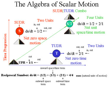
As can be seen from the chart in figure 2, since the S unit’s time progresses, and the T unit’s space progresses, there is a non-zero possibility that the two units can coincide at some point in the space/time progression. If this happens, and they combine, the resulting S|T unit’s space and time both progress, at the unit rate. Thus, the world line of the S|T unit is plotted parallel to the green diagonal line of unity.
Moreover, as indicated by the text below the chart, there are three, orthogonal “dimensions” to this combo:
1) Outward space motion (ds/dt = 1/2)
2) Outward time motion (ds/dt = 2/1)
3) Inward space/time motion (ds/dt = 1/1)
Hence, with the new concept of scalar motion, comes a new concept of scalar math, and a new concept of scalar geometry, providing the basis of a new concept of scalar science.
In the new scalar science, rotation, in the sense of changing direction, is a meaningless concept, because scalars don’t have directions. Therefore, the concept of “scalar rotation” is an oxymoron, and Larson’s entire development is based on the concept of “scalar rotation.” However, if we can manage to replace his inconsistent concept of scalar rotation, as a concept that depends upon the orthogonality of three vectorial directions, with a consistent concept of scalar expansion, as a concept that depends upon the orthogonality of three scalar “directions,” we are confident that great things can come of it.
Already, we can see results beginning to emerge from the shadows. For instance, the notion of integer and half integer spin of bosons and fermions appears to be reflected in the difference between balanced RNs and unbalanced RNs. The intimation that magnitudes of electrical charge correspond to space and time “directions” in unbalanced RNs, while they manifest as chirality in balanced RNs, also seems promising, and so on.
The work along these lines is just beginning, but Larson’s work stands as a beacon, lighting the way to what promises to be a whole new world of physics.
Ninth Post in the BAUT RST Forum
The nineth post in the BAUT forum follows. These posts are a continuation of the RST thread in the “Against the Mainstream” forum of BAUT.
+++++++++++++++++++++++++++++++++++++++++++++++++++++++++++++++++++++++++++++
What we are doing at the LRC is investigating how these multi-dimensional RNs correspond to material particles such as electrons, neutrinos, positrons, protons, neutrons, anti-protons, etc, and photons. Larson did the same thing, only he didn’t have the mathematical development that we have with the RNs.
He reasoned that the oscillations, 1/2 and 2/1, were periodic displacements; that is, that they were not “stuck” at 1/2 and 2/1, but could take on other space/time progression ratios, beginning with 1/3, or 3/1, and going to 1/4, 1/5, 1/6, … 1/n, or going from 3/1 to 4/1, 5/1, 6/1, …, n/1. The increasing values of the displacements in these time and space displacements represent lower and lower frequencies of photons (1/n), relative to the speed of light, and higher and higher frequencies of photons (n/1), relative to the speed of light.
These n speed-displacements, as he called them, on either side of unity, represented a continuous spectrum of radiation from infinitely below infrared to infinitely above ultraviolet. They are actually a discrete series of frequencies, but because they can mix and match on their way out of matter aggregates, which is their source, they appear as a continuous spectrum, unless filtered appropriately through a prism to separate them out.
Now Larson also reasoned that, since these oscillations were confined to one unit of space (ds/dt = 1/n), or one unit of time (ds/dt = n/1), which he assumed was a one-dimensional unit of space or time, these units could be rotated, like an oscillating vector can be rotated. This concept of the speed-displacements, as 1D vectorial oscillations, also enabled him to account for the propagation of the photons, because, if the oscillation were only effective in one of three dimensions, that left two dimensions in which no displacement was present (where ds/dt = 1/1 in each, undisplaced, dimension). Thus, such a photon was “free” in these two remaining dimensions; that is, it proceeded outward at unit speed, relative to a fixed refererence system, in one of these two free dimensions, which accounts for the observed outward propagation of different frequency photons, in every direction from a source, at the constant speed of light.
This was Larson’s scalar theory of radiation, if you will. If you consider that it was developed in the same time frame roughly that the quantum theory of light was being developed, during the 1930s and 1940s, when so little was known about radiation, especially among amatuer investigators, it is really an impressive model of radiation.
However, unlike traditional physicists, who were entirely focused on accounting for the energy levels of atomic spectra, using the Bohr model of the atom and traditional vector motion concepts, Larson deduced his model from first principles, by simply assuming that space is the reciprocal aspect of time in the equation of motion and nothing more.
It’s hard to imagine a more radical break from traditional physics than that which this concept represents, because it goes right to the heart of the system of physics used by centuries of physicists to account for nature, and, while they were able to calculate the energy of the atomic spectra, thanks to Heisenberg’s non-commutative product in the Taylor series, they had no idea how to explain the constant speed of light, or how to explain its spectrum of frequencies.
Indeed, they still can’t do this. In this respect, light is still a complete mystery, because while the difference in energy of the separate states of electrons in the atomic structure can be shown to correspond to the energy of the atomic spectra, using quantum mechanics, there is no understanding at all as to how this energy happens to be manifest as an oscillation, or how this oscillation, once it exists, propagates outward in every direction away from the atom, at the constant speed of light.
In contrast, Larson’s concept was consistent in this regard, but he couldn’t calculate the atomic spectra, try as he might. He finally gave up trying to solve the problem in the late 1950s, deciding to move on with his theory and to return to the problem at a later date. Of course, he never did return to it, and this has become a rather embarassing gap, or lacuna, in his theoretical development.
At the LRC, we are convinced that the reason Larson couldn’t calculate the atomic spectra values from his theory is symptomatic of a fundamental error in his development, and it is our objective to correct this error. However, while it’s easy enough to explain the error that we have found, it is a little more difficult to clarify its implications in the consequent development of the theory.
Therefore, I think that the best way to approach it is to employ Hestenes’ GA and the concepts of Clifford algebra in an effort to explain it, even though Larson knew nothing about them. Recall that GA is based on the fourth Clifford algebra, Cl3, the fourth dimension, 23 (starting with the zeroth dimension of the scalars), of the binomial expansion, or octonions, which is known as the 3D Euclidean algebra, but which mathematicians regard as eight dimensional, because 23 = 8 (whew!)
If you start from the left side of the 23 expansion, 1 3 3 1, you have four, independent, linear “vector” spaces (the space of traditional mathematics): the 20 = 1 scalar space, the 21 = 2 vector space, the 22 = 4 bivector space, and the 23 = 8 trivector space. Recall that, in GA, these four Clifford algebra spaces correspond to Euclidean geometry’s concepts of points, lines, areas, and volumes, so that the 20 space is the space of real numbers (in GA), the 21 space is the space of 1D vectors in three dimensions (therefore three, orthogonal, vectors), the 22 space is the space of 2D bivectors in three dimensions (therefore three, orthogonal, areas), and the 23 space is the space of 3D trivectors in three dimensions, which is a pseudoscalar, or an expanded point (volume). Mathematicians formulate these four, independent, linear spaces, in terms of basis vectors, written as
1) = e0;
2) = e1,e2,e3;
2) = e12, e13; e23;
4) = e123
Now, we can view Larson’s development as beginning at the left with the first linear space, the space of scalars, and proceeding to the right toward the space of trivectors; that is, we start with the unit progression, or universal expansion of space and time, where ds/dt = 1/1, a scalar, and we generate a vector through the “direction” reversals of one aspect of the scalar (ds/dt = 1/n or n/1.)
However, regarding the oscillation thus produced, as a one-dimensional oscillation, as Larson did, affects only one of the three, orthogonal vectors, in the adjoining vector space, the remaining two vectors in this space are not confined by oscillation to one unit, which accounts for the propagation of the single oscillation, relative to a fixed reference system, as explained above.
The subtle contradiction that the two, undisplaced, vectors in the vector space are therefore, by definition, scalars, not vectors, is not readily apparent when GA is not available to illuminate what is happening, but we will return to this point later. In the meantime, Larson reasoned that once a vector exists in the vector space, by virtue of the 1D oscillation in the scalar, that this vector could then be rotated, transforming it from the vector space to the adjoining bivector space to the right of the vector space. Since rotation of the vector is about the mid-point of the vector, and two such rotations are possible, the motion in the bivector space consists of two bivectors, say a^b and a^c, constituting a 2D rotation.
Rotating this compound bivector in the b^c plane, completes the compound rotations, which now consist of [(a^b + a^c) + b^c], which is equivalent to a^b^c, a trivector, in Larson’s development. Notice, however, that the rotation of the one vector, in two dimensions about the mid-point, produces the second and third vector (b and c); that is, Larson reasoned that the rotation was a displacement of a different type, a rotational displacement we would say, so that, while we start with only one vector, rotating it in two dimensions about its mid point, this is tantamount to generating two more vectors, and the wedge products of these vectors can be used to represent two rotations, one a 2D rotation, and one a 1D rotation of the 2D rotation. The concept is illustrated using GA generated graphics in figure 1 below:
Figure 1. One 2D + 1D Combination of Rotations as 3 Vectors, 3 Bivectors, and 1 Trivector
However, the problem referred to earlier, wherein, the vectors in the vector space are really not vectors, but scalars, is now exacerbated by the fact that they are transformed into vectors through displacement by rotation in the bivector space, if you will, so that they don’t become vectors directly, but indirectly, by virtue of rotation. I say that this is subtle, because it is consistent, if one considers that the initial, 1D, vibration is an object that is free to rotate as an object would, or at least, it seems to be consistent.
For instance, an extended object, such as the single blade of an aircraft propeller, rotates in a plane orthogonal to the plane of the thrust it produces, but this plane of rotation rotates as the aircraft rotates around its latitudinal axis, thus, in a sense, the combined rotation of the propeller in a given plane of rotation, and the rotation of the plane of rotation itself, is a two-dimensional rotation. Meanwhile, the compound rotation of the rotating propeller (let’s detach it from the aircraft) can also be rotated around the third axis as well.
If units of rotation are equated with units of displacement from unity, in separate scalar magnitudes in this manner, the compound rotations of figure 1 can be equated to independent 2D and 1D scalar motions, which is exactly what Larson does. In this way, he can then add and subtract various units of 1D and 2D “scalar rotation” to form composites that constitute theoretical entites, corresponding to observed physical entities such as electrons, positrons, neutrinos, protons, antiprotons, neutrons, etc, and because the non-rotated oscillation propagates at unit speed, as radiation, he has all he needs to construct the world’s first general theory of the universe, a theory of everything, so-to-speak, where the entire physical structure of the universe consists of nothing but motion.
The concepts of force, such as electrical, magnetic, and gravitational force, as properties of the constituent motions of a given theoretical entity, emerge from the development in a natural and very compelling manner. At the same time, the concepts of space and time forming this system lead to an entirely different cosmology, where the big bang concept of infinite matter/energy, expanding outward in cosmic inflation, producing the elements of matter in the process through nucleosynthesis, and aggregates of matter through gravity, which just happens to be perfectly balanced at this particular time in the evolution of the universe, so that the density of matter/energy is neither curving the spacetime fabric outward, nor inward, is replaced by an entirely new cosmology.
In the RST cosmology, the universe is cyclic, but not in the sense of a singular evolutionary process of matter/energy, dominated by laws of enthropy, but in a parallel evolutionary process dictated by the laws of motion, where the unit space/time progression produces two, inverse, sectors of the universe, constantly engaged in an eternal feedback loop.
The details of this development, as far as Larson could develop them are contained in his works, and they are amazingly consistent and compelling, much more so than the standard hot big bang cosmology, especially as more and more observations such as galaxies older than they should be in a serial type evolutionary process, and observations of gravitational anomalies that are attributed to dark matter and dark energy, etc. are made. However, there is a fly in the ointment: Larson’s concept of “scalar rotation,” upon which the whole development rests, is an oxymoron!
I’ll explain this in the next post.