The New Physics
Resolving Fundamental Issues
 6 Comments
 Email
Email Print
PrintIn discussing the RST model with Sam, I referred him to the FQXI paper that I wrote entitled “What is the Point of Reality?” which takes on the enigma and the fundamental issue of the point concept, at the heart of all physics.
The LST community covers the enigma up with “Poincaré stresses,” but truth be told, it was the reason the LHC was built: They want to resolve the issue, not just cover it up. The RST community is still striving to resolve it, as well. K.V.K. Nehru challenged Larson’s concept of “simple harmonic motion,” which Larson described as “…a motion in which there is a continuous and uniform change from outward to inward and vice versa.”
Nehru objected to the validity of this conclusion, based on the fact that scalar “directions,” inward and outward, are discrete. There is no scalar “direction” that is partly outward or partly inward. He writes:
Since there is nothing like more outward (inward) or less outward (inward) the question arises as to the meaning of the statement “a continuous and uniform change from outward to inward”? Outward and inward, as applied to scalar motion, are discrete directions: the scalar motion could be either outward or inward. There are no intermediate possibilities.
In the LRC RST-based theory (RSt), the periodic “direction” reversals are 3D, thus avoiding the saw-tooth vs. sine-wave dilemma that plagued Larson and that drove him to positing his concept of simple harmonic motion. The reversal from a 3D expansion to a 3D contraction, and vice-versa, clearly has the gradual change, to which Nehru objected, built right into it: As the expanding volume grows toward unit size, its outward rate of spherical expansion slows, even while the radius’ rate of expansion remains constant. At the point of reversal, the decrease of the volume in the inward “direction” is again gradual at first, even though the radius’ change of “direction” is instantaneous.
At the zero point (3D origin), however, this is not the case, unless we recognize the nature of the point described in the FQXI paper: In that case, the gradual change in “direction” of the spatial sphere, at one end, is matched by the gradual change in “direction” of the temporal sphere, at the other end, and, thus, it is perfectly analogous to the concept of the interchange of inverses that is inherent in rotation and also in simple harmonic motion.
Nevertheless, while 3D oscillation solves the enigma of the point, it introduces another one, an enigma that is uniquely ours: If the 3D space (time) unit oscillates by changing into its inverse, isn’t that tantamount to the numerator changing into the denominator, in the case of the SUDR, and vice-versa, in the case of the TUDR?
This question has gnawed at me ever since I wrote the FQXI paper. The tentative conclusion that I have been forced to come to is that it’s a matter of accounting. If 8 units of space are converted into 8 units of time, during an expansion to 64 units of space and 64 units of time, then the net balance is 64 - 8 = 56 units of space and 64 + 8 = 72 units of time, an 8 unit deficit of space and an 8 unit surplus of time.
During the next step, when 8 units of time are transformed into 8 units of space, the space deficit is made up from the time surplus. This is not unlike the swinging pendulum, when the potential energy is max, it’s all on one side of zero, and this surplus is transferred back to the reciprocal side, from which it came, before the cycle repeats itself.
If it works for mass, momentum and vector motion, why not for space, time and scalar motion? Maybe Ted’s quantum wave equation would be applicable after all.
:)
The Marvelous Secrets of Three Dimensions (four counting 0)
The last time I posted an entry here was exactly a year ago yesterday. It seems impossible, but that’s what the date on the previous post indicates.
To say the least, I needed something interesting to write about, before the year ends. I did post an article about the LST preon theory published in the 2012 November issue of Scientific American, but I wanted something new to write about our RST-based theory of preons (RSt). To go on record in this momentous year 2012, with something significant, something to advance the theory, just seems important.
Well, in the general discussion the other day, the fact that the LRC’s RSt, unlike Larson’s RSt and unlike Peret’s RSt, is developed using mathematics, albeit a new mathematics, as well as logic, came up and I decided that I had better go back and reread it to refresh my memory, in order to be ready to answer questions about it.
Wow, was I surprised! Here, before leaving the LRC for six months, Larry the mathematician and I had been working out the mathematics of the SUDR and its inverse the TUDR in pursuit of the properties of the preons and thus the standard model particles. I had discovered my silly mistake of using the square root of two and its inverse in this endeavor, instead of the square root of three.
Big difference. Instead of dealing with neat values with a factor of 8, we were facing a somewhat awkward factor of 27! It takes 27 volumes of a SUDR to equal the value of one TUDR! I didn’t want to believe it. I tried and tried to figure a way out of it, but finally had to resign myself to the fact that we would have to work with it.
Then, to my utter surprise, I found it confirmed in the development of the new mathematics that I had written up four or five years ago. My doubts originated from the assumption of inverse geometry, where we used the equation r’2 =r x r”, to quantize the SUDR and TUDR and found that the SUDR volume is 1/27 the volume of the TUDR. Yet, writing years before learning anything about this equation, I had come up with the exact same thing, only in terms of poles!
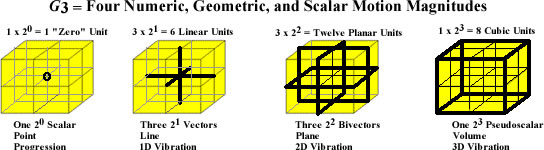
I had forgotten all about it, but counting the poles of the dimensions of the tetraktys,
1) 20 = 1
2) 20 + 21 = 3
3) 20 + 21 + 22 = 9
4) 20 + 21 + 22 + 23 = 27
the 3D line, the fourth dimension counting from 0, contains 27 poles: 1 monopole, 3 dipoles, 4 quadrupoles and 1 octopole (1 + (3x2) + (3x4) + 1(8) = 27.)
Now, how do calculations of geometric ratios, using the equations for circumference, area, and volume, all requiring the use of pi, and employing the equation of inversive geometry, in other words, the use of equations of continuous magnitudes, turn out to be identical to calculations based on fundamental numbers, dimensions and polarities (“directions”), all based on discrete quantities?
A surprise it may be, but it is the truth. Check it out for yourself, dear reader.
It turns out that the connection is the sacred number three, the union of duality, which, impressively enough, is the very definition of the Reciprocal System, the fundamental of which are embodied in Larson’s Cube.
The graphic above is outdated, but appropriate, because when I developed the new mathematics, I had yet to even think about the inner and outer circles contained by the LC and also containing it. This is all I had at the time.
I think this is a worthy announcement, a discovery to match the year 2012, and just in the nick of time too!
:)
Algebra of Tetraktys, Geometry of Larson's Cube & the Wheel of Motion
When I first showed the LRC’s RST-based “Wheel of Motion” to our new LRC associate, Larry, the mathematician, he said, “Well that’s nice, but how come you don’t make it 3D?”
I’ve always hated that question, because in a 3D universe, the periodic table of elements ought to be 3D, but the wheel of motion, like the periodic table, is only a 2D representation of the periods of its elements. It has always seemed to me that showing the true periodic nature of the elements in the wheel format, which eliminates the confusing gaps in the table format, was accomplishment enough, especially since the wheel format clearly shows the true magnitudes of the RST-based 4n2 numbers, rather than quantum mechanics (QM)-based 2n2 half-period numbers of the table.
Well, it turns out that several years ago, studying the numbers of the tetraktys, we discovered how they are actually the algebraic equivalent of the geometry of Larson’s Cube. Since then, we’ve been trying to understand the SUDR and TUDR, and their combinations as preons, which we call S|T units that combine to form the so-called “fundamental particles” of our preon version of the standard model, and connect them to the wheel. These entities combine to form the seqence of elements in the wheel, following a 4+16+36+64 = 120 pattern of mathematical “slots” for the 118 elements plus the proton and the neutron.
It’s not been easy, but we have made some progress, with many starts and stops along the way. One important connection links the progression of the LC (and thus the tetraktys) with the wheel of motion. We’ve found that we can encode the universal space/time expansion in terms of the expanding LC, which can be written as the expanding 3D level of the tetraktys
TEn = ne0 (+) 2(ne0)1 (+) 4(ne0)2 (+) 8(ne0)3
where TEn is the expanded LC equivalent of the tetraktys, n is the unit variable of its time expansion, and e0 is the scalar time unit (i.e. e0 = 1, the point, but it also represents one line, one square and one cube, after one unit of time expansion), corresponding to one edge of the LC (measured from the interior center point of the LC to the face center, lying along any one of the three axes of the stack of 8 one-unit cubes, making up the LC.)
So, in 1 unit of time, the value of TEn is
TE1 = 1*10 (+) 2*11 (+) 4*12 (+) 8*13 = 1 (+) 2 (+) 4 (+) 8
The (+) operator indicates the joining together of the four components of the LC, the respective values of the scalar point unit, the linear line unit, the square area unit, and the cubic volume unit of the LC, into one, unified, entity, isomorphic to the 3D line of the tetraktys (20, 21, 22, 23).
This is similar to the concept of joining of the scalar, vector, bivector and trivector into a multivector in Hestenes’ Geometric Algebra. Only, in our case, we join the 0D scalar and the three pseudoscalars of the tetraktys into the LC.
Hence, at t=2,
TE2 = 2e0 (+) 2(2e0)1 (+) 4(2e0)2 (+) 8(2e0)3 = 2 + 4 + 16 + 64
Similarly,
TE3 = 3 + 6 + 36 + 216,
and
TE4 = 4 + 8 + 64 + 512.
Now, clearly, any of the six 2x2 = 4 face units of the 2x2x2 = 8 stack of cube units of TE1 corresponds to the four slots of the innermost wheel of the Wheel of Motion, where the RST-based period is 4n2 = 4, when n = 1 (The four slots for the Proton, Neutron, Protium, Deuterium (H).)
Similarly, any one of the six 4x4 = 16 face units of the 4x4x4 = 64 stack of cubic units of TE2 corresponds to the sixteen slots of the second, outer wheel, when 4n2 = 16, n = 2.
The third wheel corresponds to one of the six 6x6 = 36 face units of the 6x6x6 = 216 cubic units of TE3, where the RST-based period is 4n2 = 36, n = 3, and the fourth wheel corresponds to one of the six 8x8 = 64 face units of the 8x8x8 = 512 stack of cubic units of TE4, where the RST-based period is 4n2 = 64, n = 4.
Of course, the question is, how do we know that this is anything other than a mathematical coincidence? Where is the physical connection to these numbers? Well, the answer is that we are still trying to clarify that connection, but it’s certainly interesting to note that the ratios of the associated balls of the LC follow this same numerical pattern that we see in the expanded right lines.
That is to say, the ratios of the respective radii, surfaces and volumes of the two balls associated with TE1, TE2, TE3 and TE4 (the outer ball and its inverse), follow the same numerical pattern as do the edges, lines, squares and cubes in the expanding LC, because, as it turns out, the ratio of the radius of an initial volume to that of the nth volume of equal magnitude added to it, is equal to the cube root of n. Everything follows from there.
If we take the outer ball of the LC, which geometry and algebra agree must have a radius equal to the square root of 3, and its inverse ball, which must have a radius equal to the inverse of the square root of 3, and follow their expansion as the LC expands, we find that it takes the sum of the volume of 8 balls in each case to expand the ratio of the radius of the initial ball to the radius of the nth ball from 1 to 2, (81/3 = 2).
It then takes 64 of these volumes to expand the ratio of the two radii to 4, (641/3 = 4). It takes 216 volumes to expand the ratio to 6, (2161/3 = 6), and it takes 512 volumes to expand the ratio to 8, (5121/3 = 8).
Thus, we see that there is not only a 0D, 1D, 2D and 3D mathematical (discrete unit) connection between the algebra of the tetraktys, the geometry of the LC and the Wheel of Motion, but there is also found a corresponding physical (i.e. continuous unit) connection between them.
Moreover, we see that it is the area aspect of a given volume that yields the 4n2 periods of the wheel, which means that the associated sums of the 3D volumes are actually incremented to form the 2D elemental slots in each period; That is, summing the volumes leads to the RST’s 4n2 relation, because the six faces of each expanded stack of one-unit cubes are degenerate. Thus, only one need be selected to select associated two-unit volumes. Consequently, since the smallest face possible has a magnitude of four squares, when the successive expanded LCs are divided by 4, we get the required relation:
4/4 = 12; 16/4 = 22; 36/4 = 32; 64/4 = 42.
And because this is so, we can just as easily represent the periods in the wheel as a factor of cubes:
8n3 = 8, n=1; 8n3 = 64, n= 2, 8n3 = 216, n=3; 8n3 = 512, n=4,
which is just the cubic progression of the LC.
So, to answer Larry, from a graphics perspective, it’s just much easier to draw a 2D wheel of motion than it would be to draw a 3D version. However, from a mathematical perspective, the 2D aspect of the wheel cannot be separated from its 3D aspect, because, in reality, they are simply two aspects of the same thing.
The bottom line is, even though the Wheel of Motion is not drawn in 3D, it represents a 3D volume sequence nevertheless.
Now, we need to find the way to build the expanded LCs (TE1, TE2, TE3, TE4), using the S|T units that serve as the preons to our standard model of particles. Some ideas on that next.
Heading Down the New Road
As we make the course correction discussed in the entry below, it’s useful to note that we can now view Einstein’s mass -> energy equation in terms of the SUDR/TUDR combos.
To see this, we need only change the way the equation is usually written. We change from
E = mc2,
to
E = c2 * m,
which, in space/time terms, may be written,
t/s = (s/t)2 * (t/s)3,
but this can also be written in terms of SUDR and TUDR ratios, as a ratio of their respective 2D area scalar speeds to their respective 0D radius scalar speeds, in this manner:
t/s = ((s/t)/(t/s))/((s2/t)/(t2/s))
In the reciprocal speeds of the first term, the 0D radii space units yield unit speed ratios:
s/t = 2(20)/2(20) = 2/2 = 1 and t/s = 2(20)/2(20) = 2/2 = 1,
and the physical dimensions are squared, when the inverse multiplication operation is carried out:
((s/t)/(t/s)) = ((s/t)*(s/t)) = s2/t2.
However, in the 3D term, the physical dimensions are raised up from 2D to 3D, by the inverse multiplication operation:
s3/t = 2(22)/2(20) = 8/2 and t3/s = 2(22)/2(20) = 8/2.
Hence:
((s2/t)/(t2/s)) = ((s2/t)*(s/t2)) = s3/t3,
which are the volume dimensions of inverse mass.
Consequently, when the final inverse multiplication operation is carried out, we get Einstein’s familiar equation:
t/s = (s/t)2 * (t/s)3.
The surprising thing about this, however, is that the inverse multiplication operation on the ratio of these two geometric magnitudes, equates them numerically with the next higher dimensional unit, what we might call the fundamental magnitudes of Larson’s Cube (LC), the 1D line width (21), the 2D area face (22) and the 3D volume cube (23); that is, the necessary mathematical operation of the fundamental reciprocal relation raises 2 to 4 (22 = 4) and 4 to 8 (22 * 2 = 23 = 8), and then, subsequently, the 2D area magnitude multiplied times the 3D volume magnitude is equal to the 1D line magnitude, just as it should be.
This will no doubt be really useful in working with the S|T units of the preons in terms of energy, starting with the neutrinos and working our way down to the electrons and positrons and finally combining the quarks into protons and neutrons and adding the electrons to the protons, to begin working our way up the periodic table of the elements.
But more than this, it appears that this marvelously clear insight into the meaning of the terms in Einstein’s famous equation might reduce the horribly arcane subject of modern physics to a toy model that can be taught, starting in elementary school.
Now, we need to take a look at the less famous, but more enigmatic equation of Max Planck, E = hv, in the light of the LC..
 Doug
Doug
According to the principle of Occam’s Razor, the simplest explanation is the best. In that case, then, the two terms of Einstein’s equation should be:
t/s = ((s2/t0)/(t2/s0)) * ((s3/t0)/(t3/s0))
= ((s2/t0)*(s0/t2)) * ((s3/t0)*(s0/t3))
= (s2/t2) * (s3/t3)
= c2 * m
Which is mighty straight forward: 1/2D * 3D = 1D.
Doug
Once you start making a mistake, it just keeps going on! The above equation is incorrect. The intrinsic scalar motion of matter is measured as resistance to that motion, or inertia, and that is what makes the equation work. So, when the inverse of the 3D motion of matter is used in the equation, it is correct:
t/s = ((s2/t0)/(t2/s0)) * ((s3/t0)/(t3/s0))
= ((s2/t0)*(s0/t2)) * ((s3/t0)*(s0/t3))
= (s2/t2) * (s3/t3) = s5/t5,
But substituting the dimensions of mass (inverse dimensions of matter) for the dimensions of matter, we get
(s2/t2) * (t3/s3) = t/s
While not as straight forward, it’s still clear: 1/2D * 3D = 1D
"Floundering Around in the Dark and Actually Stuck"
I just finished watching an interesting talk by Ed Witten entitled “Knots and Quantum Theory,” given at the prestigious Institute for Advanced Studies (IAS) at Princeton. Witten more or less describes his exploration of the connection that knot theory has to quantum theory, which serves to exemplify how researchers spend most of their time “floundering around in the dark,” and finding themselves “actually stuck” in their efforts to make sense out of the physical structure of the universe.
I have found the same thing in my little microcosm of theoretical physics research. Only in my case, instead of struggling to understand the monumental and vast complexity of the arcane subjects with which the intellectual giants at IAS work, I struggle to understand the straightforward first four numbers, one, two, three and four. Nevertheless, I too must admit that I spend most of my time floundering in the dark and actually stuck.
For example, for a long time I have tried to connect in my pea brain the LRC’s preon model of the so-called elementary particles of particle physics with the two balls of Larson’s cube (LC); that is, the inner and outer balls defined by the LC, the one contained by it and the one containing it.
These two balls are nested in an intriguing way that can be extended in both “directions” analogous to the way numbers can be extended in the positive and negative “directions.” I had noticed that the radius of the next smaller inner ball (in the “negative direction”), nested inside the radius of the initial inner ball, and is the inverse of the first outer ball, with the inner ball in between them representing unity (to distinguish these three balls, I will refer to them as inverse, unit and outer, from this point on) And since, presumably, this is the relationship of the unit space and unit time oscillations (SUDRs & TUDRs) used to construct the preons of our preon model, it seemed to be a natural conclusion that they could be used to quantify the SUDR and TUDR. However, so far, the attempt to proceed on this basis has only led to floundering and I have been stuck ever since.
At length, I’ve had to conclude that, in spite of tantalizing clues that this is the direction to go, I must be doing something wrong. I must not be thinking about the LC in the correct way and this has caused me to reflect on the curious observation that I made some time ago, that these balls are nothing real. The only real part of the construction is the LC itself. The balls can only exist as some sort of phantom representation of the discrete numbers of the LC. They appear as soon as the LC appears and disappear as soon as the LC disappears, even though their radii are both smaller and larger than the unit magnitude of the LC, regardless of how small or large that unit might be, ad infinitum.
Yet, what I have also known for some time is that the ratio of the inverse and outer balls is a rational number, which relates to the discrete numbers of the LC in a remarkable way, but I think I tried to use that fact in a way that that led me to equate the SUDR and TUDR with the two, inverse, balls directly, when I should have been using their ratio only.
This means that the reciprocal relationship of the SUDR and TUDR is still to be found in the original 1/2+1/1+2/1 = 4/4 equation, not in its equivalent, substituting the square root of 2 or the square root of 3 for the unit. However, both of those square roots are associated with the discrete equation in the sense that their ratio translates the discrete numbers of the LC to the continuous magnitudes of the two, inverse, balls.
For example, the numerical progression of the LC is 23 = 8, 43 = 64, 63 = 216, 83 = 512, where the base number is 2 because each dimension has two “directions,” and the exponent is 3 because there are no new phenomena beyond 3 dimensions (Bott’s periodicity theorem). But just as the LC’s volume expansion is a discrete number, the expansion of its two associated, inverse, balls is a continuous magnitude, given by the volume formula for a ball, V = 4/3 * π * r3.
Consequently, since the r of the 2D slice of the unit ball is always 1/2 of the cube root of the LC discrete number, the associated discrete progression of its radius is, 1/2*81/3 = 1, 1/2*641/3 = 2, 1/2*2161/3 = 3, 1/2*5121/3 = 4, and since the r of the 2D slice of the outer ball is always the square root of 2 times the corresponding r of the 2D slice of the unit ball, the discrete progression of its radius is 21/2 * 1 = 21/2, 21/2 * 2 = 81/2, 21/2 * 3 = 181/2, 21/2 * 4 = 321/2.
Now, the question is, what are the corresponding radii of the 2D slice of the inverse balls? The procedure that I have been trying to use depends on the assumption that this radius can be determined by geometric construction: Simply construct a new LC inside the unit ball and take the radius that fits inside it as the next lower radius in the progression. This procedure comes from the fact that each upper radius can be constructed similarly. So, how can it matter what size we choose as the unit size to relate the two inverses to?
However, as I said, this has led to floundering, even though it seems logical. I should note that it was compelling to me for at least two reasons. First, it’s easy to see that the radius of the first ball constructed in this manner is the inverse of the square root of 2, the radius of the outer ball. Second, it allows us to extend the radii in two “directions” from the unit ball, situated between these two, inverse, radii, just as the number 1/1 is situated between the two inverse numbers, 1/2 and 2/1.
In spite of these two sirens, however, I think it’s necessary to resist the temptation to go that way and instead to look at unity as the real part that must be increased. This means that we take the unit progression as 1/1, 2/2, 3/3, …n/n. While this might seem to be a trivial assumption given the fundamental postulates of the RST, the 1/2+1/1+2/1 = 4/4 equation was misleading, since it seemed to imply that the traditional number line, 1/1, 2/1, 3/1, …n/1, should be taken as representing the positive displacement values we need: To the left of 1/1, we have the increasing values of what Larson called time displacements, and to the right we have the increasing values of what he called space displacements, which are the inverse of the time displacements.
This is logical and straightforward, but perhaps it is wrong in the sense that it only succeeds in describing the inverse displacements from 2/2. After all, we can’t get any displacement from 1/1. If this is so, then the next two displacements we have to go to are at the 4/4 and the 6/6 units in the progression, and so on:
1) 2/2 = (1/2)/(1/2)
2) 4/4 = (1/4)/(1/4)
2) 6/6 = (1/6)/(1/6)
.
.
.
n) n/n = (1/n)/(1/n)
The advantage of this line of thinking over the previous is that it brings the mathematical development into conformity with the postulates, and it makes the relationship of the SUDR and TUDR to be inverse in the same sense that space and time are inverse: The quantity on the left is the inverse of the quantity on the right, by virtue of the division symbol; that is, they are not inverse numerically (i.e. both are positive), but they are inversely related in the equation, just as two opposed, but equal, 1D line segments are both positive magnitudes.
It’s also obvious that the 1 in the numerator is not the quantity 1 numerically, but it is the same number that is in the denominator, raised to the power of 3, representing 1 volume unit as a whole, expanded and contracted, as the number 1 represents one cycle of 2π radians in the LST equations. Thus, in terms of space and time dimensions, the discrete progression turned oscillation is different in each dimension. For three dimensions, the volume progression (i.e. volume frequency of oscillation, in units per cycle) is:
2*(23)/2*(20) = 8, 2*(43)/4*(20) = 32, 2*(63)/6*(20) = 72, 2*(83)/8*(20) = 128.
For two dimensions, the frequency is:
2*(22)/2*(20) = 4, 2*(42)/4*(20) = 8, 2*(62)/6*(20) = 12, 2*(82)/8*(20) = 16.
For one dimension, the frequency is:
2*(21)/2*(20) = 2, 2*(41)/4*(20) = 2, 2*(61)/6*(20) = 2, 2*(81)/8*(20) = 2,
which is constant!
To say the least, this has very encouraging implications for the preon combos, but we need continuous magnitudes, not discrete units, since nature expands (contracts) spherically, not cubically. This is where the ratio of the outer ball and its inverse comes in: It serves to translate these discrete mathematical numbers into continuous physical magnitudes, or at least that is what we hope for.
More next time.